33  Linear Transforms

33.1 Learning objective

Understand the lighting model I = aT + b as a general linear transform; see what each parameter does geometrically in pixel-value space; learn why orthogonal transforms (DFT, DCT) preserve energy while general linear transforms do not.

---

33.2 Linear transformations

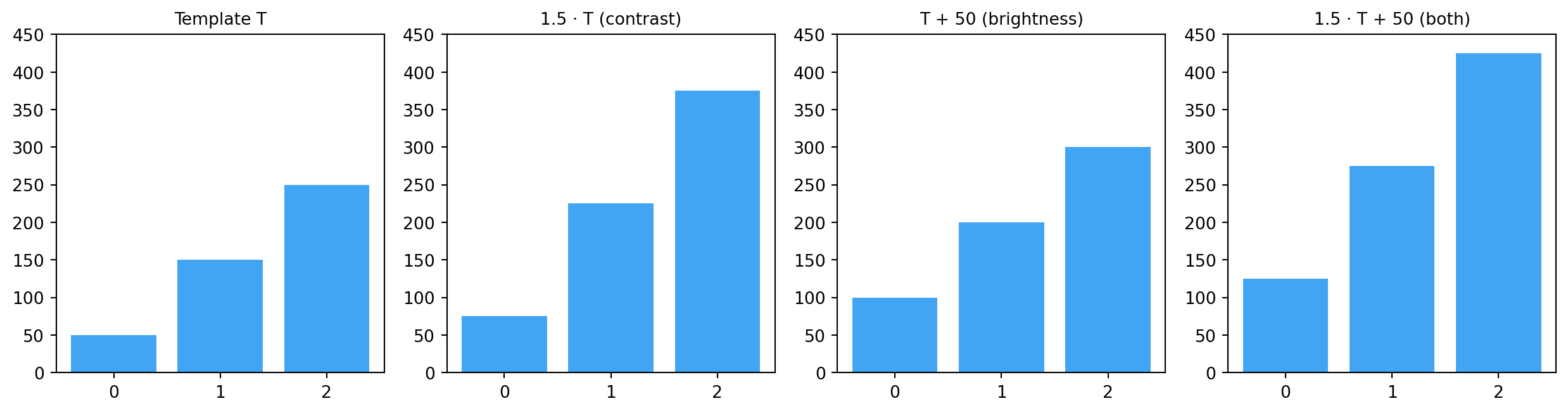
In real-world template matching, the scene patch is rarely a pixel-perfect copy of the template. Lighting changes. The relationship is modelled as a linear transform:

I \;=\; a \cdot T + b

where:

• a — contrast change (stretches/compresses the pixel spread)
• b — brightness offset (shifts all pixels up or down uniformly)

Geometrically:

• Scaling (a) multiplies the vector by a scalar. Changes the length but not the direction. Cosine similarity handles this correctly.
• Offset (b) adds b \cdot [1, 1, \ldots, 1] to the vector. Shifts the point toward the [1, 1, \ldots, 1] diagonal — changes the direction. Cosine similarity gives the wrong answer; mean subtraction is needed to undo it.

import numpy as np
import matplotlib.pyplot as plt

COLORS = {
    "primary":   "#2196F3",
    "secondary": "#4CAF50",
    "highlight": "#F44336",
    "transform": "#9C27B0",
    "gradient":  "#FF9800",
}

T = np.array([50, 150, 250], dtype=float)

fig, axes = plt.subplots(1, 4, figsize=(13, 3.5))
for ax, (vec, label) in zip(axes, [
    (T,            "Template T"),
    (T * 1.5,      "1.5 · T (contrast)"),
    (T + 50,       "T + 50 (brightness)"),
    (1.5 * T + 50, "1.5 · T + 50 (both)"),
]):
    ax.bar(range(len(vec)), vec, color=COLORS["primary"], alpha=0.85)
    ax.set_ylim(0, 450)
    ax.set_title(label, fontsize=10)
    ax.set_xticks(range(len(vec)))

plt.tight_layout()
plt.show()

---

33.3 Orthogonal transforms — energy preservation

An orthogonal transform is a special linear transform whose matrix Q satisfies:

Q^\top Q \;=\; I \quad \text{(identity)}

This means:

• The columns of Q are orthonormal (perpendicular unit vectors).
• The transform is a pure rotation (and/or reflection) — no stretching.
• Energy is preserved: \|Q\vec x\|^2 = \|\vec x\|^2.

A general linear transform \vec y = A \vec x can change the L2 norm:

\|A\vec x\| \;\neq\; \|\vec x\| \quad \text{in general}

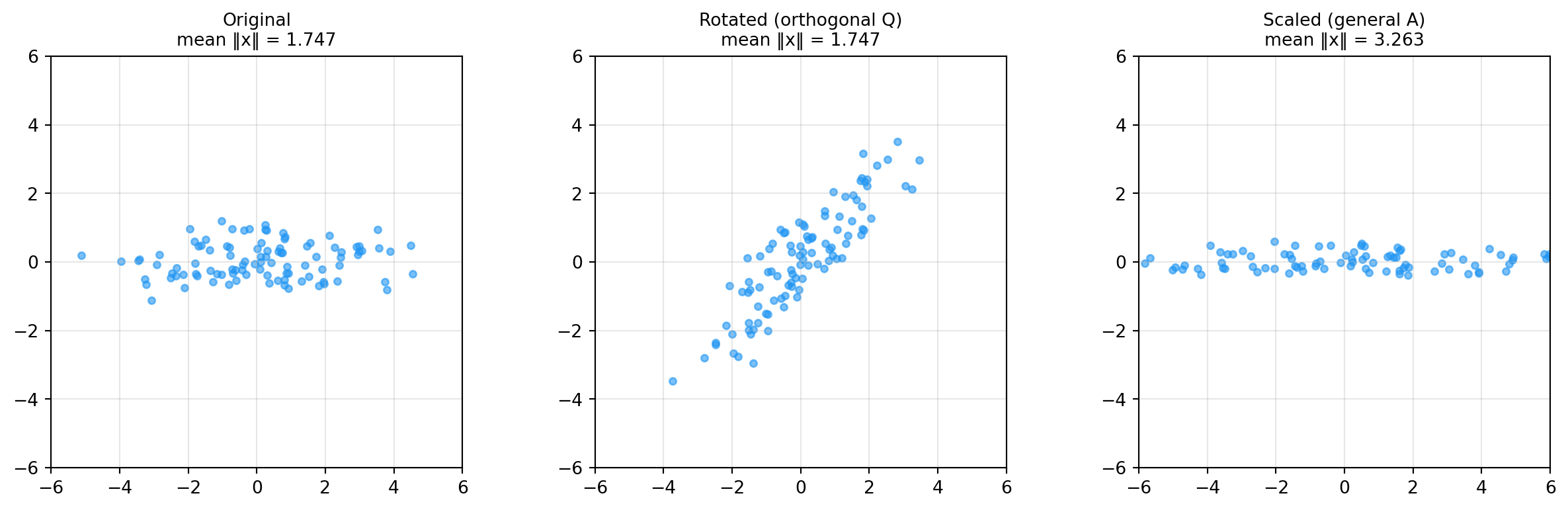
The transform distorts the signal — it stretches some directions and compresses others.

---

33.4 Parseval’s theorem

Transforms like the DFT (Discrete Fourier Transform) and DCT are orthogonal. When you transform a signal to the frequency domain, the total energy is the same — it is just redistributed across frequency bins instead of pixel positions. This is Parseval’s theorem:

\sum_{n} |x[n]|^2 \;=\; \frac{1}{N} \sum_{k} |X[k]|^2

np.random.seed(0)
x = np.random.randn(1024)
X = np.fft.fft(x)

energy_time = np.sum(np.abs(x) ** 2)
energy_freq = np.sum(np.abs(X) ** 2) / len(x)

print(f"Energy in time domain      : {energy_time:.4f}")
print(f"Energy in frequency domain : {energy_freq:.4f}")
print(f"Equal (Parseval)?          : {np.isclose(energy_time, energy_freq)}")

Energy in time domain      : 994.8747
Energy in frequency domain : 994.8747
Equal (Parseval)?          : True

---

33.5 Rotation as a literal energy-preserving transform

np.random.seed(0)
points = np.random.randn(2, 100) * np.array([[2.0], [0.5]])  # ellipse cloud

theta = np.deg2rad(45)
Q_rot = np.array([[np.cos(theta), -np.sin(theta)],
                  [np.sin(theta),  np.cos(theta)]])
A_scl = np.diag([2.0, 0.5])

rot = Q_rot @ points
scl = A_scl @ points

fig, axes = plt.subplots(1, 3, figsize=(13, 4))
for ax, (data, title) in zip(axes, [
    (points, "Original"),
    (rot,    "Rotated (orthogonal Q)"),
    (scl,    "Scaled (general A)"),
]):
    ax.scatter(data[0], data[1], s=15, alpha=0.6, color=COLORS["primary"])
    norms = np.linalg.norm(data, axis=0)
    ax.set_title(f"{title}\nmean ‖x‖ = {norms.mean():.3f}", fontsize=10)
    ax.set_aspect("equal")
    ax.set_xlim(-6, 6)
    ax.set_ylim(-6, 6)
    ax.grid(True, alpha=0.3)

plt.tight_layout()
plt.show()

A pure rotation preserves the length of every vector. A non-orthogonal scaling does not.

The rotated cloud has the same mean length as the original — the scaled cloud doesn’t.

---

33.6 The hierarchy

All transforms
  └── Linear transforms  (T(ax + by) = aT(x) + bT(y))
        ├── General linear  (energy may change)
        │     • contrast scaling:  I = 2T
        │     • brightness offset: I = T + 50
        │     • both:              I = aT + b
        │
        └── Orthogonal / Unitary  (energy preserved: ||Qx|| = ||x||)
              • rotation matrices
              • DFT, DCT
              • Hadamard transform

Linearity is necessary but not sufficient for energy preservation. Orthogonality is the additional property that guarantees it.

---

33.7 Why this matters in ML

• PCA — eigenvectors of the covariance matrix form an orthogonal basis. Projecting onto top components compresses energy into a few numbers.
• Wavelets / DCT-based codecs — JPEG works because the DCT concentrates the energy of natural patches in the low-frequency bins; quantising the rest is nearly lossless.
• Self-attention in transformers uses dot products and softmax-normalised similarities — the same machinery in higher dimensions.
• Whitening — the data is rotated so its features are decorrelated, then scaled to unit variance. Many neural nets implicitly learn similar transforms in their early layers.

---

33.8 Exercises

1. Construct a 3 \times 3 rotation matrix. Verify Q^\top Q = I.
2. Generate a random vector and rotate it 100 times by 5°. Plot the evolving point. Confirm length is preserved.
3. Apply the DCT to a 1D signal. Plot original and reconstructed signal after zeroing the top half of frequency bins. Quantify energy lost.
4. The lighting model I = aT + b has two free parameters. Find a matrix A and a vector \vec c such that I = A T + \vec c is linear (in the affine sense) and equivalent.

---

33.9 Glossary

linear transform — a function that satisfies T(a\vec x + b\vec y) = aT(\vec x) + bT(\vec y).

orthogonal matrix — square matrix Q with Q^\top Q = I; columns are orthonormal.

unitary matrix — complex generalisation of orthogonal; Q^* Q = I.

Parseval’s theorem — energy in time domain = energy in frequency domain (for orthogonal transforms).

DFT / DCT — orthogonal transforms to the frequency domain.

energy preservation — \|Q\vec x\| = \|\vec x\| for orthogonal Q.

affine transform — linear plus translation; I = aT + b.