15  Exploratory Data Analysis

15.1 The Reversal

In probability, you knew the distribution and asked: what data would it produce?

In statistics, you have the data and ask: what distribution produced it?

This reversal is the entire subject. You already understand random variables, Bernoulli trials, and what a distribution means. Now we point that knowledge at real data and ask hard questions.

---

15.2 The Question

“Everyone knows first babies are born late.”

You’ve heard this. Your parents believe it. It gets repeated at baby showers. But is it actually true? And how would you know?

This is the central question of Chapter 1 — and of statistics itself. The goal is not to trust intuition. The goal is to replace anecdote with evidence.

---

15.3 A Statistical Approach

The trap most people fall into: they remember the cases that confirm their belief and forget the ones that don’t. This is called confirmation bias, and it’s built into human cognition.

Statistics gives us a way out:

1. Find data collected independently of our belief
2. Define the question precisely (what does “late” mean?)
3. Compute something measurable
4. Decide if the difference is real or just noise

Step 4 is what most of this course is about. But first, we need data.

---

15.4 The Dataset — NSFG

The National Survey of Family Growth is a US government survey conducted by the CDC. The 2002 cycle interviewed 7,643 women aged 15–44 about their pregnancies, births, and health. It is designed to be representative of the US population.

Why this dataset?

• Large enough to detect small effects
• Collected by professionals with no agenda about first babies
• Contains exactly the variables we need: pregnancy length, birth order, birth weight

15.4.1 Key Variables

Variable	Description
caseid	Unique ID for each respondent
prglngth	Pregnancy length in weeks
outcome	1 = live birth, 2 = induced abortion, 3 = stillbirth, …
birthord	Birth order (1 = first baby, 2 = second, …)
agepreg	Mother’s age at pregnancy end (in centiyears — see below)
totalwgt_lb	Birth weight in pounds
finalwgt	Survey weight (how many women this respondent represents)

NoteWhere the data comes from

The raw .dat.gz and .dct files in data/ were downloaded once from Allen Downey’s Think Stats repository (which mirrors the CDC release). The download script is preserved as data/download_nsfg.py for reproducibility.

---

15.5 Loading the Data — From Scratch

The NSFG data comes in a fixed-width format (.dat.gz) described by a Stata dictionary file (.dct). We parse it from scratch — no helper libraries — so you see exactly what’s happening.

The .dct file has lines that look like:

_column(1)      str12      caseid     %12s    "RESPONDENT ID NUMBER"
_column(13)     byte       pregordr   %2f     "PREGNANCY ORDER (NUMBER)"

Each line tells us a column’s start position (1-indexed), Stata type, name, the number of bytes it occupies (%12s, %2f), and a label. The trailing letter — s or f — separates strings from numerics.

import re
import os
import gzip
import numpy as np
import pandas as pd
import matplotlib.pyplot as plt

# Consistent palette across all statistics chapters
COLORS = {
    "first":     "#2196F3",   # blue  — first babies
    "other":     "#4CAF50",   # green — other babies
    "highlight": "#F44336",   # red   — differences, annotations
    "neutral":   "#9E9E9E",   # grey  — background elements
}

def parse_dct(dct_path: str) -> list[dict]:
    """Read a Stata .dct file and return column specs as a list of dicts.

    Each line we care about looks like
        _column(START)  TYPE  NAME  %WIDTH(s|f)  "label"
    where START is 1-indexed and WIDTH is the column's byte width.
    """
    columns = []
    pattern = re.compile(
        r"_column\((\d+)\)\s+(\w+)\s+(\w+)\s+%(\d+)([a-z])"
    )
    with open(dct_path) as f:
        for line in f:
            match = pattern.search(line)
            if match:
                start, type_word, name, width, fmt = match.groups()
                start_idx = int(start) - 1                # 0-indexed
                end_idx = start_idx + int(width)          # exclusive
                dtype = "str" if fmt == "s" else type_word
                columns.append({
                    "name":  name,
                    "start": start_idx,
                    "end":   end_idx,
                    "dtype": dtype,
                })
    return columns


def load_fixed_width(dat_path: str, columns: list[dict]) -> pd.DataFrame:
    """Parse a gzipped fixed-width file using column specs from parse_dct."""
    records = []
    opener = gzip.open if dat_path.endswith(".gz") else open
    with opener(dat_path, "rt") as f:
        for line in f:
            record = {}
            for col in columns:
                raw = line[col["start"]:col["end"]].strip()
                if raw == "":
                    record[col["name"]] = np.nan
                elif col["dtype"].startswith("str"):
                    record[col["name"]] = raw
                else:
                    try:
                        record[col["name"]] = float(raw)
                    except ValueError:
                        record[col["name"]] = np.nan
            records.append(record)
    return pd.DataFrame(records)


data_dir = "data"
dct_path = os.path.join(data_dir, "2002FemPreg.dct")
dat_path = os.path.join(data_dir, "2002FemPreg.dat.gz")

columns = parse_dct(dct_path)
df = load_fixed_width(dat_path, columns)
print(f"Loaded: {df.shape[0]} rows × {df.shape[1]} columns")

Loaded: 13593 rows × 243 columns

Five thousand columns of survey data. We only need a handful.

---

15.6 Transformation

Raw NSFG data needs cleaning before it is usable.

15.6.1 Age in centiyears

agepreg is stored as age × 100 (e.g., 2550 means 25.5 years). We divide by 100 to get years.

15.6.2 Birth weight as pounds + ounces

birthwgt_lb and birthwgt_oz are recorded as two separate integer columns. We combine them into a single float totalwgt_lb.

df["agepreg"] = df["agepreg"] / 100.0

if "birthwgt_lb" in df.columns and "birthwgt_oz" in df.columns:
    df["totalwgt_lb"] = df["birthwgt_lb"] + df["birthwgt_oz"] / 16.0

print("Key variable ranges after transformation:")
print(f"  agepreg  : {df['agepreg'].min():.1f} – {df['agepreg'].max():.1f} years")
print(f"  prglngth : {df['prglngth'].min():.0f} – {df['prglngth'].max():.0f} weeks")

Key variable ranges after transformation:
  agepreg  : 10.3 – 44.1 years
  prglngth : -0 – 50 weeks

---

15.7 Filter to live births

outcome == 1 means live birth. Everything else (induced abortion, stillbirth, miscarriage, etc.) is a different question and we exclude it when studying birth weight and pregnancy length.

live = df[df["outcome"] == 1].copy()
print(f"Live births: {len(live):,} of {len(df):,} total pregnancies "
      f"({len(live)/len(df)*100:.1f}%)")

Live births: 9,148 of 13,593 total pregnancies (67.3%)

---

15.8 Validation — never skip this step

Before trusting any analysis, check the data against known published statistics. From the NSFG codebook:

• Total pregnancies: 13,593
• Live births: 9,148
• Mean pregnancy length (live births): ~38.6 weeks

If our numbers don’t match, something went wrong in loading or filtering.

print(f"  Total pregnancies : {len(df):,}      (expected ~13,593)")
print(f"  Live births       : {len(live):,}      (expected ~9,148)")
print(f"  Mean prglngth     : {live['prglngth'].mean():.3f} weeks  (expected ~38.6)")

  Total pregnancies : 13,593      (expected ~13,593)
  Live births       : 9,148      (expected ~9,148)
  Mean prglngth     : 38.561 weeks  (expected ~38.6)

WarningValidation is not optional

Every published bug in a statistical analysis we know of would have been caught by a check against a known number at this stage. Spend the five minutes.

---

15.9 Split by birth order

first = live[live["birthord"] == 1]
other = live[live["birthord"] > 1]

print(f"  First babies : {len(first):,}")
print(f"  Other babies : {len(other):,}")

  First babies : 4,413
  Other babies : 4,735

---

15.10 The First-Baby Effect

mean_first = first["prglngth"].mean()
mean_other = other["prglngth"].mean()
diff_weeks = mean_first - mean_other
diff_hours = diff_weeks * 7 * 24

print(f"Mean pregnancy length (first babies) : {mean_first:.3f} weeks")
print(f"Mean pregnancy length (other babies) : {mean_other:.3f} weeks")
print(f"Difference                           : {diff_weeks:.3f} weeks "
      f"= {diff_hours:.1f} hours")

Mean pregnancy length (first babies) : 38.601 weeks
Mean pregnancy length (other babies) : 38.523 weeks
Difference                           : 0.078 weeks = 13.1 hours

There is a difference. First babies are born slightly later — about 13 hours on average.

But 13 hours — is that “late”? Is it real? Could it be random noise?

These are the questions the next 13 chapters are built to answer.

---

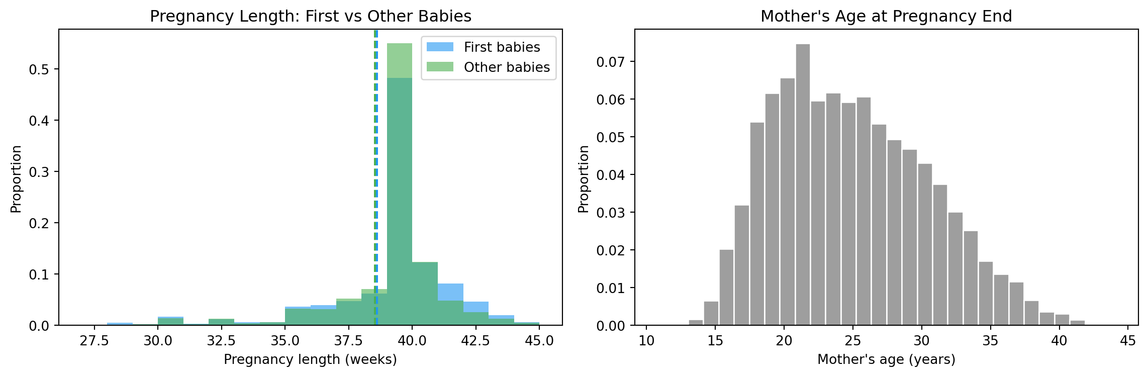
15.11 Visual first look

fig, axes = plt.subplots(1, 2, figsize=(12, 4))

# Pregnancy length: first vs other
ax = axes[0]
bins = range(27, 46)
ax.hist(first["prglngth"], bins=bins, alpha=0.6,
        color=COLORS["first"], label="First babies", density=True)
ax.hist(other["prglngth"], bins=bins, alpha=0.6,
        color=COLORS["other"], label="Other babies", density=True)
ax.axvline(mean_first, color=COLORS["first"], linestyle="--", linewidth=1.5)
ax.axvline(mean_other, color=COLORS["other"], linestyle="--", linewidth=1.5)
ax.set_xlabel("Pregnancy length (weeks)")
ax.set_ylabel("Proportion")
ax.set_title("Pregnancy Length: First vs Other Babies")
ax.legend()

# Mother's age
ax = axes[1]
ax.hist(live["agepreg"].dropna(), bins=30,
        color=COLORS["neutral"], edgecolor="white", density=True)
ax.set_xlabel("Mother's age (years)")
ax.set_ylabel("Proportion")
ax.set_title("Mother's Age at Pregnancy End")

plt.tight_layout()
plt.show()

Pregnancy length and mother’s age — the raw shapes.

The pregnancy-length histograms look almost identical. The dashed lines (the means) are close together. The 13-hour gap is buried inside the much larger spread of normal pregnancy variation.

That’s the punchline of this chapter.

---

15.12 Interpretation

The key lesson: a difference in means is just the beginning.

We need to ask:

• How large is the difference relative to the variability? (Chapter 2)
• Could this happen by chance? (Chapter 9)
• Is it practically meaningful? (Chapter 2 — effect size)

The honest answer to “are first babies born late?” turns out to be: yes, slightly, but the effect is much smaller than people believe.

Statistics doesn’t always destroy folk wisdom. Sometimes it confirms it. But it always puts a number on it — and the number usually surprises everyone.

---

15.13 Exercises

1. Load the NSFG data and print the shape of the DataFrame.
2. How many live births are in the dataset?
3. What is the mean birth weight for first babies vs others?
4. What fraction of all pregnancies result in live births?
5. Plot a histogram of agepreg for the full dataset. What shape do you see? (We’ll learn its name in Chapter 2.)

---

15.14 Glossary

anecdotal evidence — a single story or personal experience used to support a general claim.

confirmation bias — the tendency to notice and remember cases that confirm your beliefs.

DataFrame — a 2D table in pandas with named columns and an index.

outcome variable — in NSFG, the coded result of a pregnancy (live birth, abortion, etc.).

survey weight — a number that accounts for the fact that some groups were oversampled.

centiyear — one hundredth of a year; used in NSFG to store ages as integers.

validation — checking computed results against independently known values to catch errors.