“We measured 9,148 babies. But we want to say something about ALL babies. How good is our estimate?”
Everything computed so far is a sample statistic — a number computed from the data we have. What we really want is a population parameter — the true value in the real world.
The sample mean \bar{x} is our best guess for the population mean \mu. But how far off is it likely to be?
22.2 The estimation game
Suppose a population is normal with unknown \mu and \sigma. You draw a random sample of n observations. Your best estimate of \mu? The sample mean \bar{x} — the maximum likelihood estimator of \mu for a normal distribution.
Note▶ Why n-1? Bessel’s correction in one sentence
We estimated \bar{x} from the data. That used up one degree of freedom — the deviations (x_i - \bar{x}) sum to zero, so the last one is not free. Dividing by n-1 corrects for this.
For large n, the difference is negligible. For small n (say n = 5), it matters.
22.3 Sampling distributions
If you draw many samples and compute the mean of each, the distribution of those means is the sampling distribution of the mean.
Our estimate of the mean is likely within ≈ 0.015 lbs of the true mean.
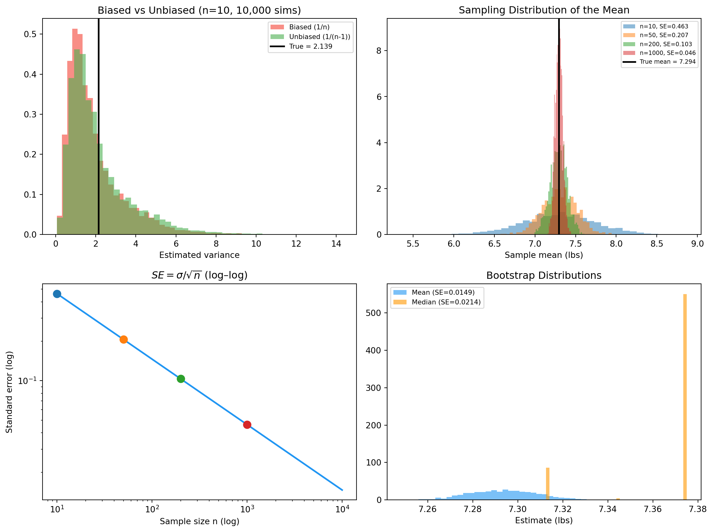
22.5 Biased vs unbiased variance — a simulation
np.random.seed(42)sample_size =10n_simulations =10_000biased, unbiased = [], []for _ inrange(n_simulations): s = np.random.choice(weights, size=sample_size, replace=False) m = s.mean() biased.append(np.sum((s - m) **2) / sample_size) unbiased.append(np.sum((s - m) **2) / (sample_size -1))true_var = weights.var()print(f"True variance : {true_var:.4f}")print(f"Mean of 1/n estimates : {np.mean(biased):.4f}")print(f"Mean of 1/(n-1) estimates : {np.mean(unbiased):.4f}")print(f"Bias 1/n : {np.mean(biased) - true_var:+.4f}")print(f"Bias 1/(n-1) : {np.mean(unbiased) - true_var:+.4f}")
True variance              : 2.1391
Mean of 1/n estimates      : 1.9136
Mean of 1/(n-1) estimates  : 2.1262
Bias 1/n                   : -0.2255
Bias 1/(n-1)               : -0.0129
The 1/n estimator is biased downward by exactly the predicted amount; the 1/(n-1) estimator is right on the nose.
22.6 SE shrinks as σ/√n
sample_sizes = [10, 50, 200, 1000]sampling = {}print(f" {'n':>6}{'SE (analytic)':>15}{'SE (simulated)':>15}")for n in sample_sizes: means = [np.random.choice(weights, size=n).mean() for _ inrange(2000)] se_a = true_std / np.sqrt(n) se_s = np.std(means) sampling[n] = (means, se_a, se_s)print(f" {n:>6}{se_a:>15.4f}{se_s:>15.4f}")
       n    SE (analytic)   SE (simulated)
      10           0.4625           0.4562
      50           0.2068           0.2095
     200           0.1034           0.1038
    1000           0.0463           0.0451
SE halves when n quadruples.
22.7 Sampling bias
Not all estimation errors are random. Bias is a systematic error that doesn’t average away with more data.
The class size paradox is a clean example: sampling students oversamples large classes, so the estimate of mean class size is biased upward — taking more data makes it more precise but not more accurate.
NSFG uses survey weights (finalwgt) to correct for deliberate oversampling of minority groups. If you ignore the weights, your estimates of national statistics will be biased.