The question
“If I know how long a pregnancy is, how well can I predict birth weight?”
Correlation (Chapter 7) told us whether two variables are related. Least squares tells us how — by fitting the best straight line through the data.
The least squares fit
We want a line \hat{y} = \alpha + \beta x that best fits the data. “Best” means minimising the sum of squared errors:
\text{SSE} \;=\; \sum_{i=1}^n (y_i - \hat{y}_i)^2
\;=\; \sum_{i=1}^n (y_i - \alpha - \beta x_i)^2
Why squared? Squaring penalises large errors more than small ones, and produces a smooth function we can minimise analytically.
Setting derivatives to zero gives the normal equations:
\hat{\beta} \;=\; \frac{\operatorname{Cov}(X, Y)}{\operatorname{Var}(X)}
\;=\; r \cdot \frac{\sigma_Y}{\sigma_X},
\qquad
\hat{\alpha} \;=\; \bar{y} - \hat{\beta}\bar{x}
The line always passes through (\bar{x}, \bar{y}).
Fit on NSFG
import sys, os
import numpy as np
import matplotlib.pyplot as plt
from scipy import stats

sys.path.insert(0, os.path.dirname(os.path.abspath("__file__")) or ".")
from _nsfg import load_groups, COLORS

live, _, _ = load_groups()

df = live[["prglngth", "totalwgt_lb"]].dropna()
df = df[(df["totalwgt_lb"] > 0) & (df["totalwgt_lb"] < 20)]
df = df[(df["prglngth"] >= 27) & (df["prglngth"] <= 44)]
x = df["prglngth"].values.astype(float)
y = df["totalwgt_lb"].values.astype(float)


def least_squares(x, y):
    cov_xy = np.mean((x - x.mean()) * (y - y.mean()))
    var_x  = np.mean((x - x.mean()) ** 2)
    beta  = cov_xy / var_x
    alpha = y.mean() - beta * x.mean()
    return alpha, beta


alpha, beta = least_squares(x, y)
print(f"Intercept α : {alpha:.4f} lbs (predicted weight at week 0 — extrapolation)")
print(f"Slope β     : {beta:.4f} lbs per week")
print(f"Each additional week adds {beta:.3f} lbs")
print(f"At 39 weeks : {alpha + beta * 39:.3f} lbs")
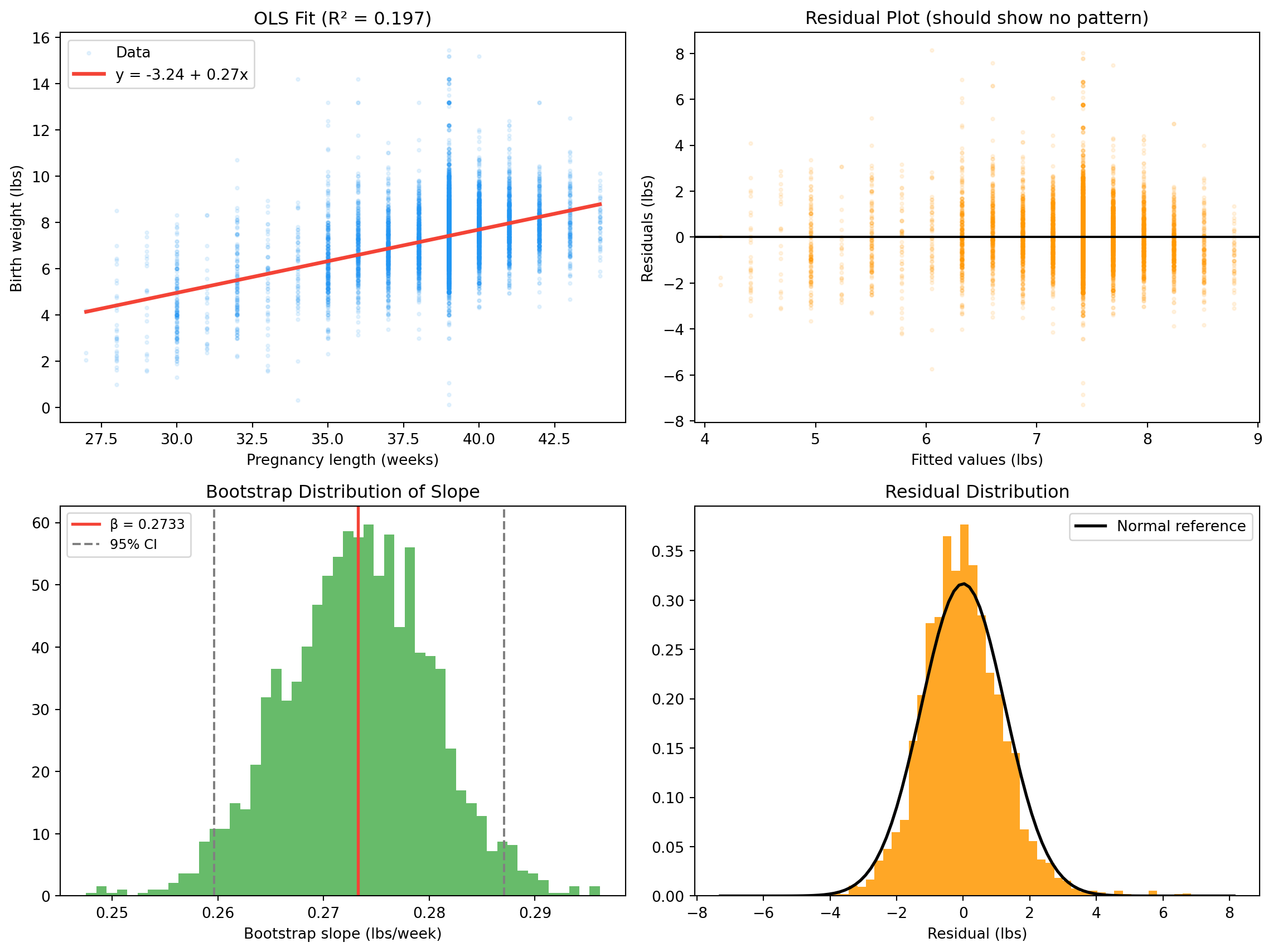
Intercept α : -3.2386 lbs (predicted weight at week 0 — extrapolation)
Slope β     : 0.2733 lbs per week
Each additional week adds 0.273 lbs
At 39 weeks : 7.418 lbs
Residuals and R^2
A residual is the difference between observed and predicted:
e_i \;=\; y_i - \hat{y}_i
A good fit has residuals that:
- Centre on zero (no systematic bias)
- Are roughly normal (for inference to work)
- Have constant variance across x (homoscedasticity)
- Show no pattern when plotted against x (otherwise the relationship is nonlinear)
The coefficient of determination R^2 measures what fraction of the variance in y is explained by the model:
R^2 \;=\; 1 - \frac{\text{SSE}}{\text{SST}},
\qquad \text{SST} = \sum (y_i - \bar{y})^2
def compute_residuals(x, y, alpha, beta):
    return y - (alpha + beta * x)


def r_squared(y, residuals):
    sse = np.sum(residuals ** 2)
    sst = np.sum((y - y.mean()) ** 2)
    return 1 - sse / sst


residuals = compute_residuals(x, y, alpha, beta)
r2 = r_squared(y, residuals)

print(f"R²              : {r2:.4f}")
print(f"Variance explained: {r2*100:.1f} %")
print(f"Residual std    : {residuals.std():.4f} lbs")
print(f"Mean residual   : {residuals.mean():.6f}  (should be ≈ 0)")
R²              : 0.1975
Variance explained: 19.7 %
Residual std    : 1.2594 lbs
Mean residual   : 0.000000  (should be ≈ 0)
Pregnancy length explains about 19 % of birth-weight variance — not a great fit. Most of the variation comes from other factors.
Bootstrap confidence interval for the slope
Is \hat{\beta} statistically meaningful? Bootstrap (Chapter 8) the slope, then read off the 2.5th and 97.5th percentile of the bootstrap distribution.
np.random.seed(42)
n_boot = 2000
boot_slopes = []
for _ in range(n_boot):
    idx = np.random.choice(len(x), size=len(x), replace=True)
    _, b = least_squares(x[idx], y[idx])
    boot_slopes.append(b)
boot_slopes = np.array(boot_slopes)
ci_lo, ci_hi = np.percentile(boot_slopes, [2.5, 97.5])

print(f"Slope          : {beta:.4f} lbs/week")
print(f"95% CI         : [{ci_lo:.4f}, {ci_hi:.4f}]")
Slope          : 0.2733 lbs/week
95% CI         : [0.2597, 0.2871]
Both bounds are positive — longer pregnancy reliably means a heavier baby.
Visualising it
fitted = alpha + beta * x

fig, axes = plt.subplots(2, 2, figsize=(12, 9))

# 1. Scatter + fit
ax = axes[0, 0]
ax.scatter(x, y, alpha=0.1, s=5, color=COLORS["first"], label="Data")
xl = np.linspace(x.min(), x.max(), 100)
ax.plot(xl, alpha + beta * xl, color=COLORS["highlight"],
        linewidth=2.5, label=f"y = {alpha:.2f} + {beta:.2f}x")
ax.set_xlabel("Pregnancy length (weeks)")
ax.set_ylabel("Birth weight (lbs)")
ax.set_title(f"OLS Fit (R² = {r2:.3f})")
ax.legend()

# 2. Residual plot
ax = axes[0, 1]
ax.scatter(fitted, residuals, alpha=0.1, s=5, color="#FF9800")
ax.axhline(0, color="black", linewidth=1.5)
ax.set_xlabel("Fitted values (lbs)")
ax.set_ylabel("Residuals (lbs)")
ax.set_title("Residual Plot (should show no pattern)")

# 3. Bootstrap distribution of slope
ax = axes[1, 0]
ax.hist(boot_slopes, bins=50, density=True, color=COLORS["other"], alpha=0.85)
ax.axvline(beta,  color=COLORS["highlight"], linewidth=2, label=f"β = {beta:.4f}")
ax.axvline(ci_lo, color="grey", linestyle="--", linewidth=1.5, label="95% CI")
ax.axvline(ci_hi, color="grey", linestyle="--", linewidth=1.5)
ax.set_xlabel("Bootstrap slope (lbs/week)")
ax.set_title("Bootstrap Distribution of Slope")
ax.legend(fontsize=9)

# 4. Residual distribution
ax = axes[1, 1]
ax.hist(residuals, bins=60, density=True, color="#FF9800", alpha=0.85)
xr = np.linspace(residuals.min(), residuals.max(), 100)
ax.plot(xr, stats.norm.pdf(xr, 0, residuals.std()),
        color="black", linewidth=2, label="Normal reference")
ax.set_xlabel("Residual (lbs)")
ax.set_title("Residual Distribution")
ax.legend()

plt.tight_layout()
plt.show()
Interpretation
- \beta is the slope: each additional week of pregnancy adds \beta pounds.
- \alpha is the intercept: predicted weight at 0 weeks (not meaningful — extrapolation).
The intercept is only meaningful within the range of observed data. Extrapolating a linear model far outside the data range is almost always wrong.
Exercises
- Fit a line predicting birth weight from pregnancy length. Report \hat{\alpha}, \hat{\beta}, R^2.
- Plot the scatter with the fitted line.
- Make a residual plot. Does the residual variance change across pregnancy lengths?
- Bootstrap the slope 1 000 times. What is the 95 % confidence interval?
- Does the slope change substantially when you use survey weights?
Glossary
least squares — minimise \sum (y_i - \hat{y}_i)^2.
slope — change in y per unit change in x.
intercept — predicted y when x = 0.
residual — y_i - \hat{y}_i.
SSE — sum of squared errors.
SST — total sum of squares.
R^2 — fraction of variance explained.
homoscedasticity — constant residual variance.
residual plot — residuals vs fitted values; key diagnostic.
extrapolation — using a model outside the observed range.