20  Probability Density Functions

20.1 From discrete to continuous

So far we’ve worked with discrete distributions (PMF) and empirical CDFs. But many real variables are conceptually continuous — birth weight, height, income.

For a continuous variable, the probability of any exact value is zero:

P(X = 7.4321\ldots) \;=\; 0

Instead, we ask: what is the probability of falling in a small interval?

P(a \leq X \leq b) \;=\; \int_a^b f(x)\, dx

Here f(x) is the probability density function (PDF). It is not a probability — it is a density. A value of f(x) = 2.5 means “probability per unit length at x is 2.5”.

---

20.2 From histogram to PDF

A histogram is an approximation of the PDF — but it depends on bin width.

The kernel density estimate (KDE) is a smooth histogram that doesn’t require you to choose bins. Instead, it places a smooth “kernel” (usually Gaussian) at each data point and sums them:

\hat{f}(x) \;=\; \frac{1}{nh} \sum_{i=1}^n K\!\left(\frac{x - x_i}{h}\right)

where h is the bandwidth (controls smoothness) and K is the kernel function.

The bandwidth is the only free parameter. Too small → noisy; too large → oversmoothed. Silverman’s rule of thumb is a good default:

h \;=\; 1.06 \cdot \hat{\sigma} \cdot n^{-1/5}

---

20.3 Building a Gaussian KDE from scratch

import sys, os
import numpy as np
import matplotlib.pyplot as plt
from scipy.stats import gaussian_kde as scipy_kde

sys.path.insert(0, os.path.dirname(os.path.abspath("__file__")) or ".")
from _nsfg import load_groups, Cdf, COLORS

live, _, _ = load_groups()
weights = live["totalwgt_lb"].dropna().values
weights = weights[(weights > 0) & (weights < 20)]


def gaussian_kernel(x, xi, h):
    z = (x - xi) / h
    return np.exp(-0.5 * z**2) / (np.sqrt(2 * np.pi) * h)


def kde(eval_points, data, h):
    densities = np.zeros(len(eval_points))
    n = len(data)
    for i, x in enumerate(eval_points):
        densities[i] = sum(gaussian_kernel(x, xi, h) for xi in data) / n
    return densities


def silverman_bandwidth(data):
    return 1.06 * data.std() * len(data) ** (-1 / 5)


h_silverman = silverman_bandwidth(weights)
print(f"Silverman bandwidth : {h_silverman:.4f} lbs")

# Use scipy on full dataset for speed; verify scratch KDE on a sample
x_eval = np.linspace(0, 16, 200)
kde_fitted = scipy_kde(weights, bw_method=h_silverman / weights.std())
kde_vals = kde_fitted(x_eval)

sample = weights[:200]
h_sample = silverman_bandwidth(sample)
x_sample_eval = np.linspace(3, 13, 100)
kde_scratch = kde(x_sample_eval, sample, h_sample)
print(f"Scratch KDE peak (n=200 sample) : "
      f"{x_sample_eval[np.argmax(kde_scratch)]:.2f} lbs "
      f"(should be near {weights.mean():.2f} lbs)")

Silverman bandwidth : 0.2505 lbs
Scratch KDE peak (n=200 sample) : 7.04 lbs (should be near 7.29 lbs)

---

20.4 The distribution framework

Now we have four ways to represent a distribution:

Representation	Answers	When to use
Histogram	rough shape	first look at data
PMF	P(X = x) for discrete X	categorical / integer data
CDF	P(X \leq x)	percentiles, comparing groups
PDF/KDE	shape of continuous distribution	smooth visualisation, modeling

They all contain the same information — just organised differently. PMF → CDF: cumulative sum. CDF → PDF: derivative. PDF → CDF: integral.

---

20.5 Moments

A moment is a summary statistic computed from powers of the data.

First (mean): \mu = E[X]

Second (variance): \sigma^2 = E[(X - \mu)^2]

Third standardised (skewness):

\text{skew} \;=\; E\!\left[\left(\frac{X - \mu}{\sigma}\right)^3\right]

• positive → long right tail
• negative → long left tail
• zero → symmetric

Fourth standardised (excess kurtosis):

\text{kurt} \;=\; E\!\left[\left(\frac{X - \mu}{\sigma}\right)^4\right] - 3

• positive (leptokurtic) → heavier tails than normal
• negative (platykurtic) → lighter tails

def skewness(data):
    mu, sigma = data.mean(), data.std()
    return np.mean(((data - mu) / sigma) ** 3)


def kurtosis(data):
    mu, sigma = data.mean(), data.std()
    return np.mean(((data - mu) / sigma) ** 4) - 3


variables = {
    "Birth weight (lbs)":       live["totalwgt_lb"].dropna().values,
    "Pregnancy length (weeks)": live["prglngth"].dropna().values,
    "Mother's age (years)":     live["agepreg"].dropna().values,
}

print(f"  {'Variable':<28}  {'Mean':>6}  {'Std':>6}  {'Skew':>7}  {'Kurt':>7}")
for name, data in variables.items():
    data = data[(data > 0) & ~np.isnan(data)]
    print(f"  {name:<28}  {data.mean():>6.2f}  {data.std():>6.2f}"
          f"  {skewness(data):>+7.3f}  {kurtosis(data):>+7.3f}")

  Variable                        Mean     Std     Skew     Kurt
  Birth weight (lbs)              7.32    2.10  +22.252  +1000.010
  Pregnancy length (weeks)       38.56    2.67   -2.629  +13.998
  Mother's age (years)           24.94    5.57   +0.422   -0.465

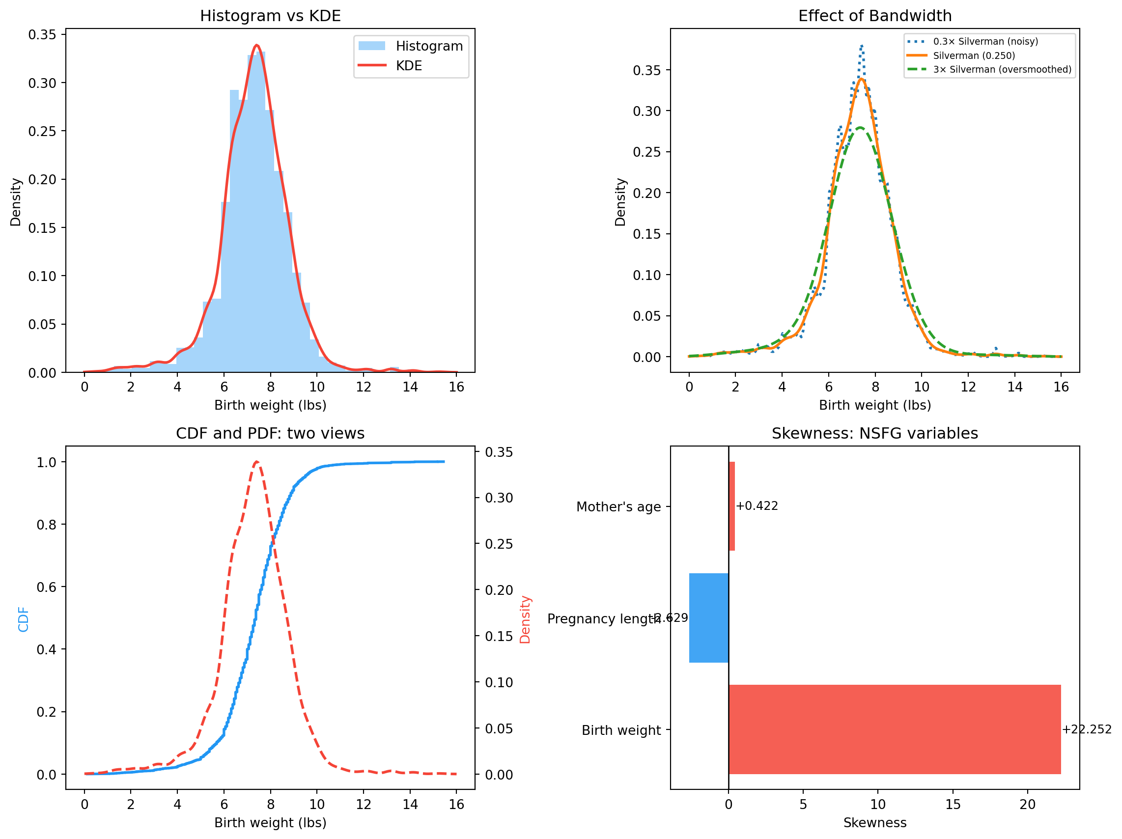
Birth weight: slight negative skew (premature babies pull the left tail down). Pregnancy length: negative (you can be very premature, but rarely very post-term). Mother’s age: slight positive skew (most mothers in their 20s, tail into the 40s).

---

20.6 Visualising it

fig, axes = plt.subplots(2, 2, figsize=(12, 9))

# 1. Histogram + KDE
ax = axes[0, 0]
ax.hist(weights, bins=40, density=True, alpha=0.4,
        color=COLORS["first"], label="Histogram")
ax.plot(x_eval, kde_vals, color=COLORS["highlight"], linewidth=2, label="KDE")
ax.set_xlabel("Birth weight (lbs)")
ax.set_ylabel("Density")
ax.set_title("Histogram vs KDE")
ax.legend()

# 2. Bandwidth effect
ax = axes[0, 1]
for h_factor, style, label in [(0.3, ":", "0.3× Silverman (noisy)"),
                                (1.0, "-", f"Silverman ({h_silverman:.3f})"),
                                (3.0, "--", "3× Silverman (oversmoothed)")]:
    h = h_silverman * h_factor
    kd = scipy_kde(weights, bw_method=h / weights.std())
    ax.plot(x_eval, kd(x_eval), linestyle=style, linewidth=2, label=label)
ax.set_xlabel("Birth weight (lbs)")
ax.set_ylabel("Density")
ax.set_title("Effect of Bandwidth")
ax.legend(fontsize=7)

# 3. CDF and PDF, two views of the same distribution
ax = axes[1, 0]
wgt_cdf = Cdf(weights)
ax2 = ax.twinx()
ax.plot(wgt_cdf.xs, wgt_cdf.ps, color=COLORS["first"], linewidth=2, label="CDF")
ax2.plot(x_eval, kde_vals, color=COLORS["highlight"],
         linewidth=2, linestyle="--", label="PDF (KDE)")
ax.set_xlabel("Birth weight (lbs)")
ax.set_ylabel("CDF", color=COLORS["first"])
ax2.set_ylabel("Density", color=COLORS["highlight"])
ax.set_title("CDF and PDF: two views")

# 4. Skewness across variables
ax = axes[1, 1]
skew_vals, names = [], []
for name, data in variables.items():
    data = data[(data > 0) & ~np.isnan(data)]
    skew_vals.append(skewness(data))
    names.append(name.split("(")[0].strip())
colors_skew = [COLORS["highlight"] if s > 0 else COLORS["first"] for s in skew_vals]
bars = ax.barh(names, skew_vals, color=colors_skew, alpha=0.85)
ax.axvline(0, color="black", linewidth=1)
ax.set_xlabel("Skewness")
ax.set_title("Skewness: NSFG variables")
for bar, val in zip(bars, skew_vals):
    ax.text(val + 0.01 if val >= 0 else val - 0.01,
            bar.get_y() + bar.get_height() / 2,
            f"{val:+.3f}", va="center",
            ha="left" if val >= 0 else "right", fontsize=9)

plt.tight_layout()
plt.show()

Histogram + KDE, bandwidth comparison, CDF/PDF on the same axes, and skewness across NSFG variables.

---

20.7 Exercises

1. Plot a KDE for birth weight at three bandwidths. How does the shape change?
2. Compute skewness for birth weight, pregnancy length, and mother’s age.
3. Which NSFG variable has the most positive skewness? The most negative?
4. Plot the CDF and its derivative (approximate PDF) for birth weight on the same figure.
5. Implement a Gaussian KDE from scratch using the kernel formula above.

---

20.8 Glossary

PDF — f(x) such that P(a \leq X \leq b) = \int_a^b f(x)\,dx.

density — value of f(x); not a probability.

KDE — smooth empirical PDF estimated from data.

bandwidth — smoothing parameter in KDE; controls noise vs smoothness.

Silverman’s rule — default bandwidth h = 1.06 \hat\sigma n^{-1/5}.

moment — E[X^k].

skewness — third standardised moment; measures asymmetry.

kurtosis — fourth standardised moment; measures tail heaviness.