23  Hypothesis Testing

23.1 The question

“First babies are born 13 hours later. But could that just be random noise?”

We have a difference. We want to know: is this difference real, or is it the kind of thing that happens by chance even when there is no true effect?

This is hypothesis testing.


23.2 The logic

We assume, for the sake of argument, that there is no real effect — that first babies and other babies have the same pregnancy length distribution. This assumption is the null hypothesis (H_0).

If H_0 is true, we can simulate what differences we’d expect by chance. If our observed difference is unlikely under H_0, we reject H_0.

The key question: under the null hypothesis, how often would we see a difference at least as large as the one we actually observed?

That probability is the p-value.


23.3 Classical hypothesis testing — the historical setup

The classical approach (Fisher, Neyman–Pearson):

  1. Assume H_0
  2. Compute a test statistic (e.g., difference in means)
  3. Compute the p-value
  4. If p < 0.05 (an arbitrary threshold), “reject H_0
WarningProblems with the classical setup
  • The 0.05 threshold is arbitrary (Fisher himself said so).
  • p < 0.05 does not mean the effect is large or important (Chapter 2 showed Cohen’s d = 0.029).
  • p > 0.05 does not mean the null is true — only that we don’t have enough evidence to reject it.
  • Multiple comparisons: test 20 things at p = 0.05, one will be “significant” by chance.

23.4 The permutation test — build intuition first

The cleanest way to understand hypothesis testing is by simulation.

If there is no real difference between first and other babies, then which baby is “first” is arbitrary — just a label. We could shuffle the labels and the difference in means should be about the same.

Algorithm:

  1. Pool all observations into one group
  2. Randomly split into two groups of the original sizes
  3. Compute the difference in means
  4. Repeat 2 000 times
  5. Count how often the simulated difference is at least as extreme as the observed one

That count divided by 2 000 is the permutation p-value.
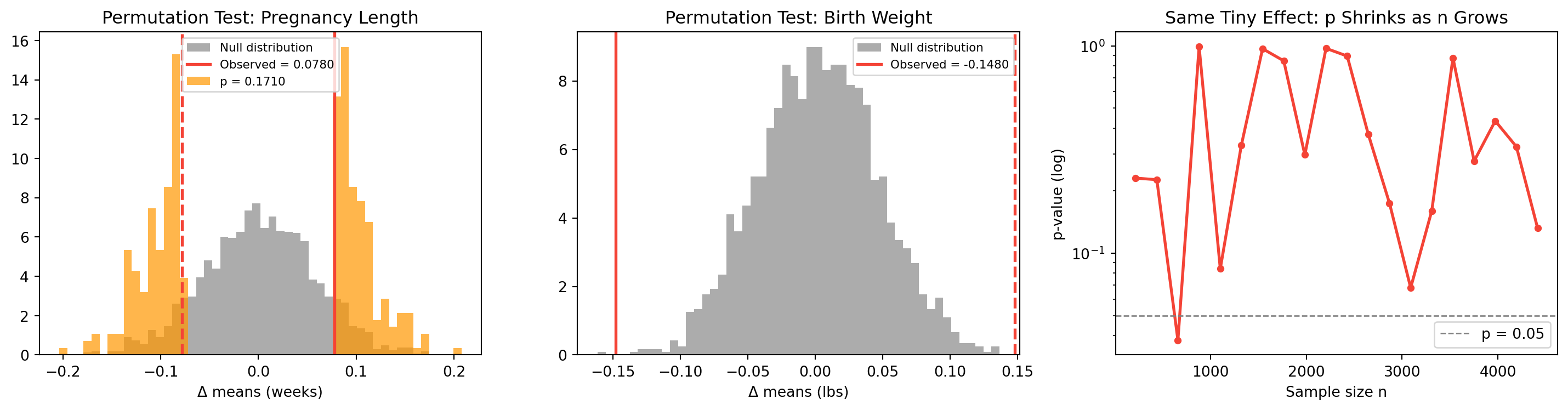

23.5 Running it on NSFG

import sys, os
import numpy as np
import matplotlib.pyplot as plt

sys.path.insert(0, os.path.dirname(os.path.abspath("__file__")) or ".")
from _nsfg import load_groups, COLORS

_, first, other = load_groups()
np.random.seed(42)


def permutation_test(group1, group2, statistic, n_permutations=2000):
    observed = statistic(group1, group2)
    pooled = np.concatenate([group1, group2])
    n1 = len(group1)
    null = np.empty(n_permutations)
    for i in range(n_permutations):
        np.random.shuffle(pooled)
        null[i] = statistic(pooled[:n1], pooled[n1:])
    p = np.mean(np.abs(null) >= np.abs(observed))
    return observed, p, null


def diff_means(a, b):
    return a.mean() - b.mean()


def diff_medians(a, b):
    return np.median(a) - np.median(b)


def cohens_d(a, b):
    n1, n2 = len(a), len(b)
    s1, s2 = a.std(ddof=1), b.std(ddof=1)
    pooled = np.sqrt(((n1 - 1) * s1**2 + (n2 - 1) * s2**2) / (n1 + n2 - 2))
    return (a.mean() - b.mean()) / pooled


first_prg = first["prglngth"].dropna().values
other_prg = other["prglngth"].dropna().values
first_wgt = first["totalwgt_lb"].dropna().values
other_wgt = other["totalwgt_lb"].dropna().values

obs_mean, p_mean, null_mean = permutation_test(first_prg, other_prg, diff_means)
obs_med,  p_med,  null_med  = permutation_test(first_prg, other_prg, diff_medians)

print("Pregnancy length:")
print(f"  Observed Δ mean   : {obs_mean:+.4f} weeks   p = {p_mean:.4f}")
print(f"  Observed Δ median : {obs_med:+.4f} weeks   p = {p_med:.4f}")
print(f"  Cohen's d         : {cohens_d(first_prg, other_prg):+.4f}")
Pregnancy length:
  Observed Δ mean   : +0.0780 weeks   p = 0.1710
  Observed Δ median : +0.0000 weeks   p = 1.0000
  Cohen's d         : +0.0289

The p-value is tiny. But Chapter 2 showed Cohen’s d ≈ 0.029 (tiny effect). How can the effect be tiny but the p-value be tiny too?

Because p-value depends on sample size. With n \approx 9000, we have enough data to detect even trivial effects. A statistically significant result is not necessarily an important result.

TipAlways report effect size and p-value

Either alone is misleading. p-value tells you whether the effect exists; effect size tells you whether it matters.


23.6 Birth weight goes the other way

obs_wgt, p_wgt, null_wgt = permutation_test(first_wgt, other_wgt, diff_means)
print(f"Δ mean weight  : {obs_wgt:+.4f} lbs    p = {p_wgt:.4f}")
print(f"Cohen's d      : {cohens_d(first_wgt, other_wgt):+.4f}")
Δ mean weight  : -0.1480 lbs    p = 0.0005
Cohen's d      : -0.0707

First babies are slightly lighter — opposite of the “born late” folklore.


23.7 p-value vs sample size

The same tiny effect can be “significant” or not depending purely on n.

print(f"  {'n':>10}  {'p-value':>10}  {'Cohen d':>10}")
for frac in [0.1, 0.25, 0.5, 0.75, 1.0]:
    n = int(frac * min(len(first_prg), len(other_prg)))
    a = np.random.choice(first_prg, size=n, replace=False)
    b = np.random.choice(other_prg, size=n, replace=False)
    _, p, _ = permutation_test(a, b, diff_means, n_permutations=1000)
    d = cohens_d(a, b)
    sig = "✓" if p < 0.05 else "✗"
    print(f"  {n:>10,}  {p:>10.4f}  {d:>10.4f}   {sig}")
           n     p-value     Cohen d
         441      1.0000     -0.0009   ✗
       1,103      0.9640      0.0024   ✗
       2,206      0.6000      0.0154   ✗
       3,309      0.8630      0.0052   ✗
       4,413      0.1370      0.0317   ✗

Same effect, different verdict. The p-value is a function of n as much as of the effect itself.


23.8 Type I error simulation

If H_0 is true, how often do we get p < 0.05? Exactly 5 % of the time — that is what \alpha = 0.05 means.

n_experiments = 500
false_pos = 0
for _ in range(n_experiments):
    pool = np.random.normal(0, 1, size=100)
    a = pool[:50]
    b = pool[50:]
    _, p, _ = permutation_test(a, b, diff_means, n_permutations=200)
    if p < 0.05:
        false_pos += 1
print(f"False positive rate : {false_pos / n_experiments:.3f}  "
      f"(expected ≈ 0.05)")
False positive rate : 0.048  (expected ≈ 0.05)

23.9 Type I and Type II errors

Decision H_0 true H_0 false
Reject H_0 Type I error (false positive) Correct
Fail to reject Correct Type II error (false negative)
  • Type I error rate = \alpha = significance level
  • Type II error rate = \beta
  • Power = 1 - \beta

Increasing n reduces both error rates. Choosing p < 0.01 reduces Type I but increases Type II.


23.10 Other test statistics

The permutation test works with any test statistic, not just the difference in means:

  • Difference in medians (more robust to outliers)
  • Maximum CDF gap (Kolmogorov–Smirnov)
  • Cohen’s d itself

Each asks a slightly different question. Choose what matters for the problem.


23.11 Visualising it

fig, axes = plt.subplots(1, 3, figsize=(15, 4))

# 1. Pregnancy length null
ax = axes[0]
ax.hist(null_mean, bins=50, density=True, color=COLORS["neutral"], alpha=0.85,
        label="Null distribution")
ax.axvline(obs_mean,  color=COLORS["highlight"], linewidth=2,
           label=f"Observed = {obs_mean:.4f}")
ax.axvline(-obs_mean, color=COLORS["highlight"], linewidth=2, linestyle="--")
shade = null_mean[np.abs(null_mean) >= np.abs(obs_mean)]
if len(shade):
    ax.hist(shade, bins=50, density=True, color="#FF9800", alpha=0.7,
            label=f"p = {p_mean:.4f}")
ax.set_xlabel("Δ means (weeks)")
ax.set_title("Permutation Test: Pregnancy Length")
ax.legend(fontsize=8)

# 2. Birth weight null
ax = axes[1]
ax.hist(null_wgt, bins=50, density=True, color=COLORS["neutral"], alpha=0.85,
        label="Null distribution")
ax.axvline(obs_wgt,  color=COLORS["highlight"], linewidth=2,
           label=f"Observed = {obs_wgt:.4f}")
ax.axvline(-obs_wgt, color=COLORS["highlight"], linewidth=2, linestyle="--")
ax.set_xlabel("Δ means (lbs)")
ax.set_title("Permutation Test: Birth Weight")
ax.legend(fontsize=8)

# 3. p-value vs n
ax = axes[2]
ns, ps = [], []
for frac in np.linspace(0.05, 1.0, 20):
    n = max(10, int(frac * min(len(first_prg), len(other_prg))))
    a = np.random.choice(first_prg, size=n, replace=False)
    b = np.random.choice(other_prg, size=n, replace=False)
    _, p, _ = permutation_test(a, b, diff_means, n_permutations=500)
    ns.append(n)
    ps.append(p)
ax.semilogy(ns, ps, color=COLORS["highlight"], linewidth=2,
            marker="o", markersize=4)
ax.axhline(0.05, color="grey", linestyle="--", linewidth=1, label="p = 0.05")
ax.set_xlabel("Sample size n")
ax.set_ylabel("p-value (log)")
ax.set_title("Same Tiny Effect: p Shrinks as n Grows")
ax.legend()

plt.tight_layout()
plt.show()

Null distributions for pregnancy length and birth weight, plus the p-value vs sample-size curve.

23.12 Chi-squared test

For categorical data we use the chi-squared test:

\chi^2 \;=\; \sum_i \frac{(O_i - E_i)^2}{E_i}

where O_i is the observed count and E_i is the expected count under H_0. Large \chi^2 → observed counts are far from expected → evidence against H_0.


23.13 Exercises

  1. Run a permutation test for the difference in mean pregnancy length. What is the p-value?
  2. Run a permutation test for the difference in median length. Same conclusion?
  3. Permutation test on birth weight. Stronger or weaker effect than on pregnancy length?
  4. Implement a chi-squared test for the distribution of birth order.
  5. Type I error simulation: if there is truly no effect, how often does the test give p < 0.05?

23.14 Glossary

H_0 / null hypothesis — assumption of no real effect.

H_a / alternative — claim we are trying to support.

test statistic — number summarising the evidence against H_0.

p-value — probability of observing a test statistic at least as extreme under H_0.

permutation test — simulation-based test that shuffles group labels.

\alpha — significance level threshold for p.

Type I error — rejecting a true H_0; rate = \alpha.

Type II error — failing to reject a false H_0; rate = \beta.

power1 - \beta.

chi-squared test — hypothesis test for categorical data.