The whole probability ladder we’ve built — Bernoulli → Binomial → Poisson → Normal, glued together by the CLT — exists to answer one question that every signal-processing engineer faces:
Given a measurement, how much of what I’m seeing is signal and how much is noise — and what shape does that noise take?
This chapter assembles the answer for the cleanest end-to-end example: the camera sensor.
10.1 The measurement chain — generic template
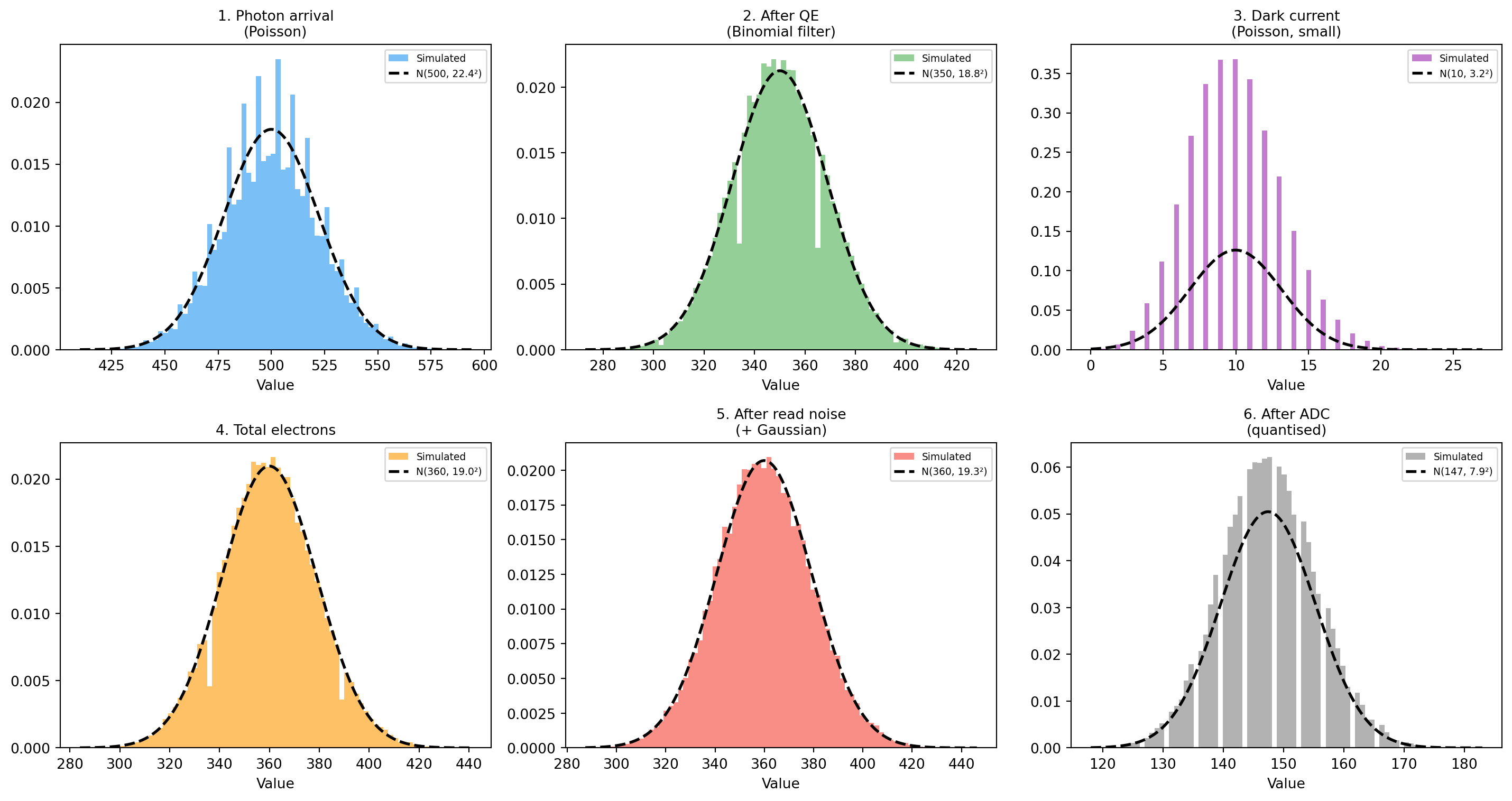
Almost every digital sensor performs the same five-stage transformation from physical world to integer reading:
physical event  →  transduction  →  accumulation  →  electronics  →  ADC
   (random)        (each event has    (sum over          (read,         (round
                    detection prob)    exposure)         amplify)        to bits)
Each stage adds its own statistical character:
Stage
Random source
Distribution
Physical event
Quantum / thermal / arrival
Poisson
Transduction
Detection probability
Binomial thinning
Accumulation
Sum over a window
Poisson stays Poisson; small-noise sums become Normal
Electronics
Amplifier and circuit noise
Gaussian (CLT on micro-disturbances)
ADC
Rounding to nearest bit
Uniform over one quantization step
The total reading is the sum of all of these, and by the CLT the sum is approximately Gaussian at moderate-to-high signal levels — which is why classical denoising tools assume Gaussian noise and get away with it.
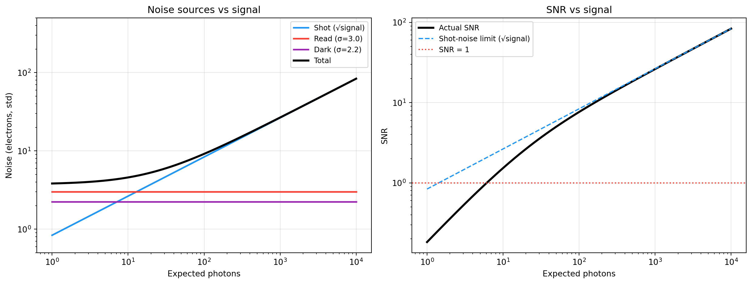
Left: noise sources vs signal. Read-noise dominates dark; shot noise dominates mid-tones; saturation kills SNR. Right: actual SNR follows the shot-noise limit between the two.
Knowing the regime tells you the right denoising strategy:
Saturation — information is irreversibly lost; no algorithm recovers it.
10.6 The same template for other sensors
Once you’ve internalised the camera example, every other sensor falls into the same template with different physics in each slot.
Vibration sensor (accelerometer):
Stage
Camera
Vibration
Physical event
Photon arrivals (Poisson)
Mechanical impacts (Poisson when bearing is faulty)
Transduction
Quantum efficiency
Piezoelectric coupling efficiency
Accumulation
Photons over exposure
Acceleration over a sample interval
Electronics
Amplifier + read noise (Gaussian)
Charge amplifier + ADC noise (Gaussian)
ADC
2^{\text{bits}} levels
2^{\text{bits}} levels
Network telemetry:
Stage
Network
Physical event
Packet drops (Poisson)
Transduction
Probability the drop is observed
Accumulation
Drops counted per minute
No analog stage, but the Poisson → Normal transition still happens as the count per window grows.
10.7 Key takeaways
Bernoulli → Binomial → Poisson → Normal is a chain of increasing abstraction. Each is a limiting case of the one before it.
Rare-event counting is Poisson — across all domains. Variance-equals-mean (\sigma^2 = \lambda) means noise is signal-dependent.
The CLT is why Gaussian assumptions work everywhere. Aggregated readings, smoothed signals, calibration averages — all converge to Normal regardless of where they started.
Every classical signal-processing algorithm that assumes Gaussian noise is implicitly relying on this entire chain. Wiener, Kalman, least-squares, learned denoisers — all sit on top of Bernoulli → Binomial → Poisson → Normal.
The three regimes — electronics-limited, physics-limited, saturated — exist in every sensor. The names change but the structure is identical.
10.8 Exercises
Run simulate_sensor for \lambda \in \{5, 50, 500, 5000\}. For each, plot the digital-value distribution and overlay a Gaussian fit. At what \lambda does the Gaussian fit visually fail?
Reduce \sigma_r by a factor of 10. Where does the read-noise → shot-noise crossover move?
Implement a frame-averaging denoiser. Show that read-noise std drops as \sigma_r / \sqrt n but shot noise drops only as \sqrt{\lambda / n}.
Pick a non-camera sensor (microphone, RF, vibration) and write out the same five-stage table for it.
10.9 Glossary
signal chain — the sequence of physical and electronic stages between a physical event and a digital reading.