8.1 An applied scenario — the silent vibration sensor
Switch the motor off. The accelerometer keeps streaming, and even though there’s nothing to measure, the readings aren’t exactly zero — they wander around it.
A few seconds of these “silent” samples produce a tight cloud centred on 0\,\mathrm{g}:
A handful of samples sit near \pm 0.001\,\mathrm{g}
Most cluster tightly around 0
Almost none stray past \pm 0.005\,\mathrm{g}
The cloud is symmetric and bell-shaped. There’s no obvious physical “rare event” being counted here — instead, every reading is a sum of dozens of tiny disturbances: thermal noise in the amplifier, electromagnetic pickup, ADC quantization, mechanical vibration from the building. None of them dominates; they just add up.
When that’s the situation — many small independent contributions summed together — the resulting distribution has a name, and a shape you’ve already glimpsed in the Binomial and Poisson plots.
8.2 Intuition
Look back at the Binomial plots. As n grew, the distribution started looking like a smooth bell curve. The Poisson does the same as \lambda grows. Sums of many small noise sources do the same thing — that’s the silent-sensor cloud above.
The Normal distribution (Gaussian) is the continuous bell-shaped curve that all of these converge to. It’s the most important distribution in statistics, signal processing, and machine learning — not because nature is “secretly Gaussian”, but because anything that’s a sum of many small independent things ends up Gaussian. We’ll prove this in the next chapter — the Central Limit Theorem.
The Normal shows up wherever sums show up:
Sensor noise floors — many independent micro-disturbances
Filter outputs — convolution averages many input samples
Calibration errors — repeated measurements of the same quantity
Aggregated metrics — mean of a batch, sum over a window
Pixel intensities in uniform regions — independent noise per pixel
\sigma^2 — variance (width of the bell); \sigma is the standard deviation
Unlike Binomial and Poisson (which are discrete — only integer counts), the Normal is continuous — it assigns probability density to any real number.
Once you’ve decided a process is Normal, the entire distribution is captured by two numbers. Almost every classical signal-processing or denoising algorithm — Wiener filtering, Kalman filtering, Gaussian blur, BM3D — assumes its inputs or noise are Gaussian.
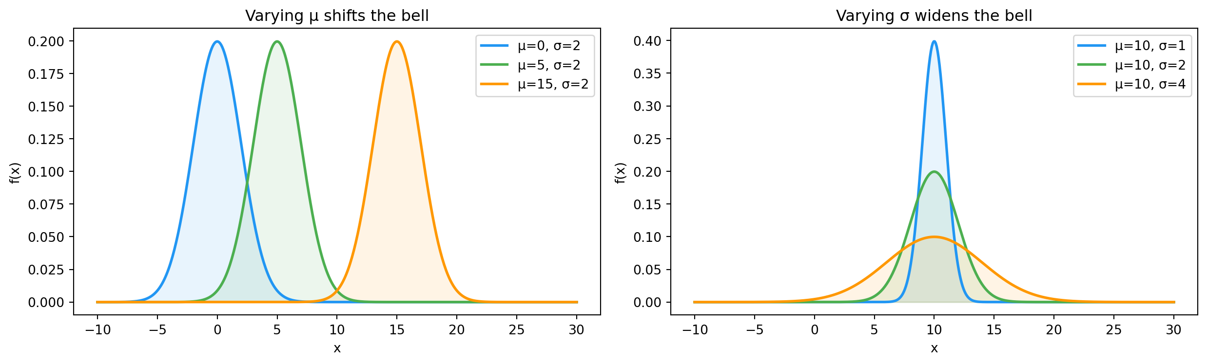
8.4 What the parameters do
import numpy as npimport matplotlib.pyplot as pltfrom scipy.stats import norm, poissonnp.random.seed(42)fig, axes = plt.subplots(1, 2, figsize=(13, 4))x = np.linspace(-10, 30, 500)ax = axes[0]for mu, color in [(0, "#2196F3"), (5, "#4CAF50"), (15, "#FF9800")]: sigma =2 pdf = norm.pdf(x, mu, sigma) ax.plot(x, pdf, linewidth=2, color=color, label=f"μ={mu}, σ={sigma}") ax.fill_between(x, pdf, alpha=0.1, color=color)ax.set_title("Varying μ shifts the bell")ax.set_xlabel("x")ax.set_ylabel("f(x)")ax.legend()ax = axes[1]for sigma, color in [(1, "#2196F3"), (2, "#4CAF50"), (4, "#FF9800")]: mu =10 pdf = norm.pdf(x, mu, sigma) ax.plot(x, pdf, linewidth=2, color=color, label=f"μ={mu}, σ={sigma}") ax.fill_between(x, pdf, alpha=0.1, color=color)ax.set_title("Varying σ widens the bell")ax.set_xlabel("x")ax.set_ylabel("f(x)")ax.legend()plt.tight_layout()plt.show()
\mu is “where is the signal?”. \sigma is “how noisy is it?”. Total area under any curve is exactly 1.
8.5 Back to the silent sensor
Fit a Gaussian to the silent-sensor samples and you’ll get something like:
\mu \approx 0,\qquad \sigma \approx 0.002 \quad \text{(both in g)}
That single number \sigma is your noise floor — the irreducible spread of the sensor when there’s no signal. Any future “signal” you measure has to be large enough relative to \sigma to be distinguishable from this floor.
Anything more than a few \sigma from the mean is suspicious: under a Normal model, |x - \mu| > 3\sigma happens about 0.27\,\% of the time. If you start seeing 5\sigma excursions on the silent sensor, the noise model itself has changed.
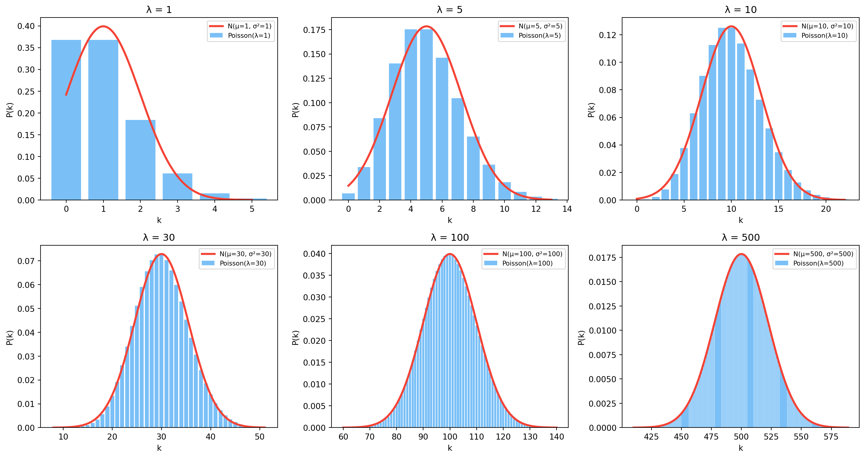
8.6 Poisson → Normal as \lambda grows
For large \lambda, the Poisson distribution is well-approximated by a Normal with the same mean and variance:
λ = 1 is clearly not Gaussian; λ = 30 is a good fit; λ = 500 is indistinguishable.
Practical threshold: for \lambda > 30, the Normal approximation is tight enough for most engineering purposes. This is why Wiener, Kalman, NLM, BM3D get away with assuming Gaussian noise — at moderate-to-high signal levels, Poisson has already become Gaussian.
Each arrow is a mathematical limit that simplifies the model while preserving the essential statistics. The next chapter shows why the Normal sits at the end of this chain — and why it’s the end of the chain for almost every other distribution too. That’s the Central Limit Theorem.
8.8 Exercises
For Normal(0, 1), verify by simulation that 68 % / 95 % / 99.7 % of samples fall within 1, 2, 3 standard deviations.
Fit a Normal to the silent-sensor data of your own (or to np.random.normal(0, 0.002, 5000)). Plot the histogram and overlay the fitted PDF.
At what value of \lambda does Poisson(\lambda) fit Normal(\lambda, \lambda) within KS distance 0.02?
Show that summing two independent Gaussians gives a Gaussian (use simulation). What are its mean and variance?
8.9 Glossary
Normal / Gaussian distribution — continuous bell-shaped distribution with mean \mu and std \sigma.
\mu, \sigma — mean and standard deviation.
density — value of f(x); not a probability.
68–95–99.7 rule — fractions of probability within 1, 2, 3 std of the mean.
noise floor — Gaussian spread of a sensor when no signal is present.