28  Analytic Methods

28.1 The question

“We’ve been simulating everything. When can we use formulas instead?”

All previous chapters built understanding through simulation — we shuffled, resampled, generated. But many textbooks give you formulas directly. When are those formulas valid? And when does simulation win?

---

28.2 Normal distributions — the special case

Many analytic results only hold when the data is normally distributed. If X \sim N(\mu, \sigma^2) and Y \sim N(\nu, \tau^2) independently, then

X + Y \;\sim\; N(\mu + \nu, \sigma^2 + \tau^2)

Sums of normals are normal. This is special — it doesn’t hold for most distributions.

---

28.3 Sampling distributions — the key results

If we draw samples of size n from a population with mean \mu and std \sigma:

\bar{X} \;\sim\; N\!\left(\mu, \frac{\sigma^2}{n}\right) \quad \text{(exactly if population is normal)}

For two samples:

\bar{X}_1 - \bar{X}_2 \;\sim\; N\!\left(\mu_1 - \mu_2, \frac{\sigma_1^2}{n_1} + \frac{\sigma_2^2}{n_2}\right)

This is how the classical two-sample t-test is derived.

---

28.4 The Central Limit Theorem (CLT)

The most important theorem in statistics.

Statement: for any population with finite mean \mu and variance \sigma^2, as n \to \infty:

\frac{\bar{X} - \mu}{\sigma / \sqrt{n}} \;\xrightarrow{d}\; N(0, 1)

The sample mean is approximately normally distributed, regardless of the shape of the population distribution, as long as n is large enough.

“Large enough” depends on skewness:

• Symmetric population → n \approx 30 usually fine
• Moderately skewed → n \approx 100
• Heavily skewed → n \approx 500+

Why does this matter? It is the reason normal-based formulas work in so many situations even when the data is not normal — we’re taking means of large samples, and means are approximately normal.

---

28.5 Watching the CLT happen

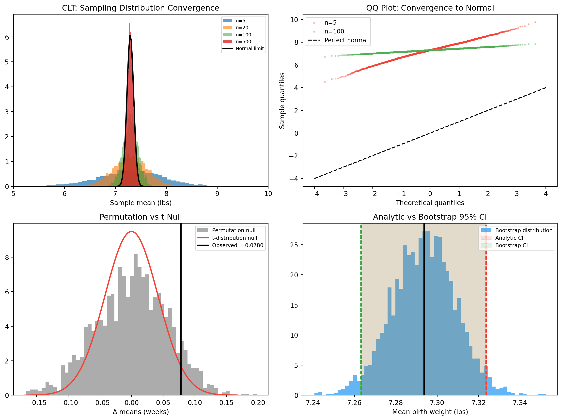
Birth weight is left-skewed (premature babies). Draw samples of increasing size and watch the sampling distribution converge to normal.

import sys, os
import numpy as np
import matplotlib.pyplot as plt
from scipy import stats

sys.path.insert(0, os.path.dirname(os.path.abspath("__file__")) or ".")
from _nsfg import load_groups, COLORS

live, first, other = load_groups()
np.random.seed(42)

weights = live["totalwgt_lb"].dropna().values
weights = weights[(weights > 0) & (weights < 20)]

first_prg = first["prglngth"].dropna().values
other_prg = other["prglngth"].dropna().values

sample_sizes = [5, 20, 100, 500]
n_samples = 5000
sampling = {}

print(f"Population: mean={weights.mean():.3f}, "
      f"std={weights.std():.3f}, skew={stats.skew(weights):.3f}")
print()
print(f"  {'n':>6}  {'mean of means':>14}  {'std of means':>14}  "
      f"{'σ/√n':>8}  {'skew':>8}")
for n in sample_sizes:
    sm = np.array([np.random.choice(weights, size=n).mean()
                   for _ in range(n_samples)])
    sampling[n] = sm
    se_theory = weights.std() / np.sqrt(n)
    print(f"  {n:>6}  {sm.mean():>14.4f}  {sm.std():>14.4f}"
          f"  {se_theory:>8.4f}  {stats.skew(sm):>+8.4f}")

Population: mean=7.294, std=1.463, skew=-0.254

       n   mean of means    std of means      σ/√n      skew
       5          7.2863          0.6513    0.6541   -0.1975
      20          7.2937          0.3380    0.3270   -0.0521
     100          7.2962          0.1446    0.1463   +0.0003
     500          7.2936          0.0654    0.0654   +0.0049

std(means) matches the theoretical \sigma / \sqrt n to multiple decimals. The skewness goes to zero — the sampling distribution becomes symmetric and normal-shaped.

---

28.6 Two-sample t-test vs permutation test

For the first-baby pregnancy length question we ran a permutation test in Chapter 9. The classical alternative is the Welch’s t-test:

t \;=\; \frac{\bar{x}_1 - \bar{x}_2} {\sqrt{s_1^2/n_1 + s_2^2/n_2}}

with Welch–Satterthwaite degrees of freedom. Under H_0, this follows a t-distribution.

def two_sample_ttest(g1, g2):
    n1, n2 = len(g1), len(g2)
    m1, m2 = g1.mean(), g2.mean()
    s1, s2 = g1.std(ddof=1), g2.std(ddof=1)
    se = np.sqrt(s1**2 / n1 + s2**2 / n2)
    t = (m1 - m2) / se
    num = (s1**2/n1 + s2**2/n2)**2
    den = (s1**2/n1)**2/(n1-1) + (s2**2/n2)**2/(n2-1)
    df = num / den
    p = 2 * stats.t.sf(abs(t), df=df)
    return t, p


def permutation_test(g1, g2, n_permutations=2000):
    obs = g1.mean() - g2.mean()
    pooled = np.concatenate([g1, g2])
    n1 = len(g1)
    null = np.empty(n_permutations)
    for i in range(n_permutations):
        np.random.shuffle(pooled)
        null[i] = pooled[:n1].mean() - pooled[n1:].mean()
    return obs, np.mean(np.abs(null) >= np.abs(obs)), null


t_stat, p_t = two_sample_ttest(first_prg, other_prg)
obs_diff, p_perm, null_perm = permutation_test(first_prg, other_prg)

print(f"Observed difference : {obs_diff:.4f} weeks")
print(f"t-test  p-value     : {p_t:.6f}")
print(f"Permutation p-value : {p_perm:.4f}")

Observed difference : 0.0780 weeks
t-test  p-value     : 0.168528
Permutation p-value : 0.1730

With large n, the two methods agree — that’s the CLT validating the t-test.

---

28.7 Analytic CI vs bootstrap CI

Using the CLT directly:

\text{CI}_{95\%} \;=\; \bar{x} \pm 1.96 \cdot \frac{s}{\sqrt n}

n = len(weights)
mean_w = weights.mean()
se_w   = weights.std() / np.sqrt(n)
z = stats.norm.ppf(0.975)
ci_analytic = (mean_w - z * se_w, mean_w + z * se_w)

boot_means = np.array([np.random.choice(weights, size=n, replace=True).mean()
                       for _ in range(3000)])
ci_boot = (np.percentile(boot_means, 2.5), np.percentile(boot_means, 97.5))

print(f"Sample mean         : {mean_w:.4f} lbs")
print(f"Standard error      : {se_w:.6f} lbs")
print(f"Analytic 95% CI     : [{ci_analytic[0]:.4f}, {ci_analytic[1]:.4f}]")
print(f"Bootstrap 95% CI    : [{ci_boot[0]:.4f}, {ci_boot[1]:.4f}]")

Sample mean         : 7.2936 lbs
Standard error      : 0.015345 lbs
Analytic 95% CI     : [7.2636, 7.3237]
Bootstrap 95% CI    : [7.2631, 7.3233]

Identical to four decimals.

---

28.8 Analytic correlation test

For Pearson’s r under H_0: \rho = 0:

t \;=\; \frac{r\sqrt{n - 2}}{\sqrt{1 - r^2}} \;\sim\; t_{n - 2}

mask = (~live["agepreg"].isna()) & (~live["totalwgt_lb"].isna())
sub = live.loc[mask, ["agepreg", "totalwgt_lb"]]
sub = sub[(sub["totalwgt_lb"] > 0) & (sub["totalwgt_lb"] < 20)]
age_c = sub["agepreg"].values
wgt_c = sub["totalwgt_lb"].values

r, p_corr = stats.pearsonr(age_c, wgt_c)
n_corr = len(age_c)
t_corr = r * np.sqrt(n_corr - 2) / np.sqrt(1 - r**2)

print(f"Pearson r    : {r:+.4f}")
print(f"t-statistic  : {t_corr:+.4f}")
print(f"p-value      : {p_corr:.6f}")

Pearson r    : +0.0684
t-statistic  : +6.5313
p-value      : 0.000000

---

28.9 Visualising it

fig, axes = plt.subplots(2, 2, figsize=(12, 9))

# 1. CLT
ax = axes[0, 0]
xrange = np.linspace(5, 10, 200)
for n, alpha in [(5, 0.7), (20, 0.6), (100, 0.5), (500, 0.8)]:
    sm = sampling[n]
    ax.hist(sm, bins=60, density=True, alpha=alpha, label=f"n={n}")
sm500 = sampling[500]
ax.plot(xrange, stats.norm.pdf(xrange, sm500.mean(), sm500.std()),
        color="black", linewidth=2, label="Normal limit")
ax.set_xlabel("Sample mean (lbs)")
ax.set_title("CLT: Sampling Distribution Convergence")
ax.legend(fontsize=7)
ax.set_xlim(5, 10)

# 2. QQ plots
ax = axes[0, 1]
for n, color in [(5, COLORS["highlight"]), (100, COLORS["other"])]:
    sm = sampling[n]
    (osm, osr), _ = stats.probplot(sm, dist="norm")
    ax.scatter(osm, osr, s=3, alpha=0.3, color=color, label=f"n={n}")
ax.plot([-4, 4], [-4, 4], "k--", linewidth=1.5, label="Perfect normal")
ax.set_xlabel("Theoretical quantiles")
ax.set_ylabel("Sample quantiles")
ax.set_title("QQ Plot: Convergence to Normal")
ax.legend(fontsize=9)

# 3. permutation null vs t-distribution null
ax = axes[1, 0]
ax.hist(null_perm, bins=60, density=True, color=COLORS["neutral"],
        alpha=0.85, label="Permutation null")
trange = np.linspace(-4, 4, 200)
df_apx = min(len(first_prg), len(other_prg)) - 1
scale = first_prg.std() / np.sqrt(len(first_prg))
ax.plot(trange * scale, stats.t.pdf(trange, df=df_apx) / scale,
        color=COLORS["highlight"], linewidth=2, label="t-distribution null")
ax.axvline(obs_diff, color="black", linewidth=2,
           label=f"Observed = {obs_diff:.4f}")
ax.set_xlabel("Δ means (weeks)")
ax.set_title("Permutation vs t Null")
ax.legend(fontsize=8)

# 4. Analytic vs bootstrap CI
ax = axes[1, 1]
ax.hist(boot_means, bins=60, density=True, color=COLORS["first"], alpha=0.7,
        label="Bootstrap distribution")
ax.axvline(mean_w, color="black", linewidth=2)
for lo, hi, label, color in [
    (ci_analytic[0], ci_analytic[1], "Analytic CI",  COLORS["highlight"]),
    (ci_boot[0],     ci_boot[1],     "Bootstrap CI", COLORS["other"]),
]:
    ax.axvspan(lo, hi, alpha=0.15, color=color, label=label)
    ax.axvline(lo, color=color, linestyle="--", linewidth=1.5)
    ax.axvline(hi, color=color, linestyle="--", linewidth=1.5)
ax.set_xlabel("Mean birth weight (lbs)")
ax.set_title("Analytic vs Bootstrap 95% CI")
ax.legend(fontsize=8)

plt.tight_layout()
plt.show()

CLT convergence, QQ plots, permutation null vs t-distribution null, and analytic vs bootstrap CI.

---

28.10 When to use which

Use simulation (permutation, bootstrap) when:

1. The data is heavily skewed or has outliers (CLT hasn’t kicked in yet)
2. The test statistic is not the mean (e.g., median, max, ratio)
3. You have small samples (n < 30)
4. The analytic formula requires assumptions you can’t verify

Use analytic methods when:

1. n is large and data is not extremely skewed
2. You need speed (simulation is 1000× slower)
3. You want closed-form confidence intervals
4. You need to communicate to an audience that expects p-values and t-statistics

---

28.11 Course summary

Across 14 chapters we’ve used the same NSFG dataset to build the core of statistics from scratch:

• Chapters 1–2: real data, histograms, effect sizes
• Chapters 3–6: PMF, CDF, modelling, PDF
• Chapter 7: relationships and correlation
• Chapters 8–9: estimation and hypothesis testing — by simulation
• Chapters 10–11: regression, multiple and logistic
• Chapters 12–13: time series and survival
• Chapter 14: when formulas replace simulation

The simulation-first arc is deliberate. Once you have built a permutation test or a bootstrap from scratch, the formulas in this chapter feel like shortcuts — special cases of the simulation that work when n is large. That’s the right mental model.

---

28.12 Exercises

1. Simulate the CLT: draw samples of size n = 5, 20, 100, 500 from birth weight. Plot sampling distributions of the mean.
2. Run a two-sample t-test for pregnancy length. Compare to the permutation test p-value.
3. Compute the analytic 95 % CI for mean birth weight. Compare to the bootstrap CI.
4. Test the correlation between age and birth weight analytically. Same result as the permutation test?
5. For which NSFG variable does the sampling distribution of the mean converge slowest to normal? Why?

---

28.13 Glossary

CLT — sample mean is approximately normal for large n.

t-distribution — sampling distribution of the mean when \sigma is unknown; → normal as n \to \infty.

t-test — hypothesis test based on the t-statistic.

Welch’s approximation — degrees of freedom for two-sample t-test without equal-variance assumption.

chi-squared distribution — distribution of \sum (O - E)^2/E under H_0 for categorical data.

analytic method — formula-based result derived from probability theory.

normal approximation — using a normal to approximate the sampling distribution when CLT applies.

convergence in distribution — a sequence of distributions approaching a limit distribution.