27 Survival Analysis

27.1 The question

“How long until a woman has her next pregnancy?”

This is a different kind of question. It is about time until an event — and some women in the dataset haven’t had the event yet. They are still “waiting”.

This is the survival analysis problem, and it requires special methods.

27.2 The problem with ignoring censoring

Suppose we just take the mean time between pregnancies for women who had two or more. This ignores the women who only had one pregnancy by the time of the survey.

But those women might go on to have more pregnancies later — we just don’t know yet. They are censored: we know they survived past time t, but we don’t know when (or if) the event occurs.

Ignoring censored observations biases the estimate downward — we only use the fast pregnancies and throw away information about the slow ones.

27.3 Survival function

The survival function S(t) is the probability of surviving past time t — i.e., the event has not occurred by time t:

S(t) \;=\; P(T > t) \;=\; 1 - F(t)

where F(t) is the CDF of event times. For inter-pregnancy intervals, S(12) = 0.6 means 60 % of women have not had their next pregnancy within 12 months.

The survival function always starts at S(0) = 1 and decreases toward 0.

27.4 Hazard function

The hazard function h(t) is the instantaneous rate of the event occurring at time t, given that it hasn’t occurred yet:

h(t) \;=\; \lim_{\Delta t \to 0} \frac{P(t \leq T < t + \Delta t \mid T \geq t)}{\Delta t} \;=\; \frac{f(t)}{S(t)}

Intuitively: if you’ve survived to t, how likely are you to have the event in the next small interval?

27.5 Building intervals from NSFG

import sys, os
import numpy as np
import pandas as pd
import matplotlib.pyplot as plt

sys.path.insert(0, os.path.dirname(os.path.abspath("__file__")) or ".")
from _nsfg import load_pregnancy_data, COLORS

preg_df = load_pregnancy_data()


def compute_intervals(df: pd.DataFrame) -> pd.DataFrame:
    """For each woman, compute gaps between consecutive pregnancies.

    Women with only one recorded pregnancy are censored — they may
    have more later, we just don't know.
    """
    if "datend" not in df.columns:
        # synthetic fallback for demonstration
        np.random.seed(42)
        n_women = 3000
        rows = []
        for i in range(n_women):
            n_preg = np.random.choice([1, 2, 3, 4], p=[0.4, 0.35, 0.18, 0.07])
            times = sorted(np.random.uniform(0, 120, n_preg))
            for j in range(len(times) - 1):
                rows.append({"caseid": i, "interval": times[j+1] - times[j],
                             "censored": False})
            if n_preg == 1:
                rows.append({"caseid": i, "interval": np.nan, "censored": True})
        return pd.DataFrame(rows)

    rows = []
    for caseid, group in df.groupby("caseid"):
        sg = group.sort_values("datend").dropna(subset=["datend"])
        dates = sg["datend"].values
        if len(dates) < 2:
            rows.append({"caseid": caseid, "interval": np.nan, "censored": True})
        else:
            for i in range(len(dates) - 1):
                rows.append({"caseid": caseid,
                             "interval": dates[i+1] - dates[i],
                             "censored": False})
            rows.append({"caseid": caseid, "interval": np.nan, "censored": True})
    return pd.DataFrame(rows)


intervals_df = compute_intervals(preg_df)
n_total    = len(intervals_df)
n_observed = intervals_df[~intervals_df["censored"]]["interval"].notna().sum()
n_censored = intervals_df["censored"].sum()

print(f"Total records      : {n_total:,}")
print(f"Observed intervals : {n_observed:,}")
print(f"Censored           : {n_censored:,}  ({n_censored/n_total*100:.1f}%)")

observed = intervals_df[~intervals_df["censored"]]["interval"].dropna().values
print(f"Naive mean (ignoring censored) : {observed.mean():.2f} months")

Total records      : 13,329
Observed intervals : 8,296
Censored           : 5,033  (37.8%)
Naive mean (ignoring censored) : 36.66 months

The naive mean systematically underestimates the true mean because women with longer intervals are over-represented in the censored group.

27.6 Kaplan–Meier estimator

The Kaplan–Meier (KM) estimator computes the survival function from data, correctly handling censored observations.

At each event time t_j:

\hat{S}(t_j) \;=\; \hat{S}(t_{j-1}) \cdot \left(1 - \frac{d_j}{n_j}\right)

where d_j is the number of events at t_j and n_j is the number still at risk just before t_j.

The key trick: censored observations contribute to n_j for all times before their censoring, but don’t contribute to d_j — they reduce the at-risk count without being counted as events.

def kaplan_meier(intervals, censored):
    t = intervals.copy()
    if np.any(np.isnan(t)):
        max_t = np.nanmax(t[~np.isnan(t)])
        t[np.isnan(t)] = max_t * 2

    event_times = np.sort(np.unique(t[~censored]))
    S = 1.0
    survival_times = [0.0]
    survival_probs = [1.0]
    for tj in event_times:
        n_at_risk = np.sum(t >= tj)
        d_j = np.sum((t == tj) & (~censored))
        if n_at_risk > 0 and d_j > 0:
            S *= 1 - d_j / n_at_risk
        survival_times.append(tj)
        survival_probs.append(S)
    return np.array(survival_times), np.array(survival_probs)


t_all = intervals_df["interval"].values.copy().astype(float)
c_all = intervals_df["censored"].values
max_obs = np.nanmax(t_all)
t_filled = np.where(np.isnan(t_all), max_obs * 2, t_all)

km_times, km_S = kaplan_meier(t_filled, c_all)

print(f"  {'Months':>8}  {'S(t)':>8}  Meaning")
for cp in [6, 12, 18, 24, 36]:
    idx = np.searchsorted(km_times, cp)
    if idx < len(km_S):
        s = km_S[idx]
        print(f"  {cp:>8}  {s:>8.3f}  "
              f"{(1-s)*100:.1f}% have had next pregnancy by month {cp}")

    Months      S(t)  Meaning
         6     0.965  3.5% have had next pregnancy by month 6
        12     0.899  10.1% have had next pregnancy by month 12
        18     0.801  19.9% have had next pregnancy by month 18
        24     0.716  28.4% have had next pregnancy by month 24
        36     0.597  40.3% have had next pregnancy by month 36

27.7 Hazard from survival

def hazard_from_survival(times, survival):
    h_times, h_vals = [], []
    for i in range(1, len(times)):
        dt = times[i] - times[i - 1]
        if dt > 0 and survival[i - 1] > 0:
            h = -(survival[i] - survival[i - 1]) / (survival[i - 1] * dt)
            h_times.append(times[i])
            h_vals.append(h)
    return np.array(h_times), np.array(h_vals)


h_times, h_vals = hazard_from_survival(km_times, km_S)
print(f"Computed hazard at {len(h_times)} time points.")

Computed hazard at 205 time points.

27.8 Visualising it

fig, axes = plt.subplots(2, 2, figsize=(12, 9))

# 1. Naive vs KM
ax = axes[0, 0]
naive_sorted = np.sort(observed[observed < 60])
n = len(naive_sorted)
naive_S = 1 - np.arange(1, n + 1) / n
ax.step(naive_sorted, naive_S, color=COLORS["highlight"], linewidth=2,
        where="post", label="Naive (ignores censoring)")
mask = km_times <= 60
ax.step(km_times[mask], km_S[mask], color=COLORS["first"], linewidth=2,
        where="post", label="Kaplan-Meier")
ax.set_xlabel("Months since last pregnancy")
ax.set_ylabel("S(t) = P(no next pregnancy yet)")
ax.set_title("Survival Curve")
ax.legend(fontsize=9)
ax.set_xlim(0, 60)

# 2. Hazard
ax = axes[0, 1]
smooth = pd.Series(h_vals).rolling(5, center=True, min_periods=1).mean().values
mh = h_times <= 60
ax.plot(h_times[mh], smooth[mh], color="#9C27B0", linewidth=2)
ax.set_xlabel("Months")
ax.set_ylabel("Hazard rate")
ax.set_title("Hazard Function h(t)")
ax.set_xlim(0, 60)

# 3. Distribution of observed intervals
ax = axes[1, 0]
clip = observed[(observed > 0) & (observed < 72)]
ax.hist(clip, bins=30, density=True, color=COLORS["first"], alpha=0.85)
ax.axvline(np.median(clip), color=COLORS["highlight"], linewidth=2,
           label=f"Median = {np.median(clip):.1f} months")
ax.set_xlabel("Inter-pregnancy interval (months)")
ax.set_ylabel("Density")
ax.set_title("Observed Intervals\n(censored excluded — biased!)")
ax.legend(fontsize=9)

# 4. Observed vs censored
ax = axes[1, 1]
labels = ["Observed\n(event)", "Censored\n(no event yet)"]
counts = [n_observed, n_censored]
colors = [COLORS["first"], COLORS["neutral"]]
bars = ax.bar(labels, counts, color=colors, alpha=0.85)
for b, c in zip(bars, counts):
    ax.text(b.get_x() + b.get_width() / 2, b.get_height() + 20,
            f"{c:,}", ha="center", fontsize=10)
ax.set_ylabel("Count")
ax.set_title("Observed vs Censored")

plt.tight_layout()
plt.show()

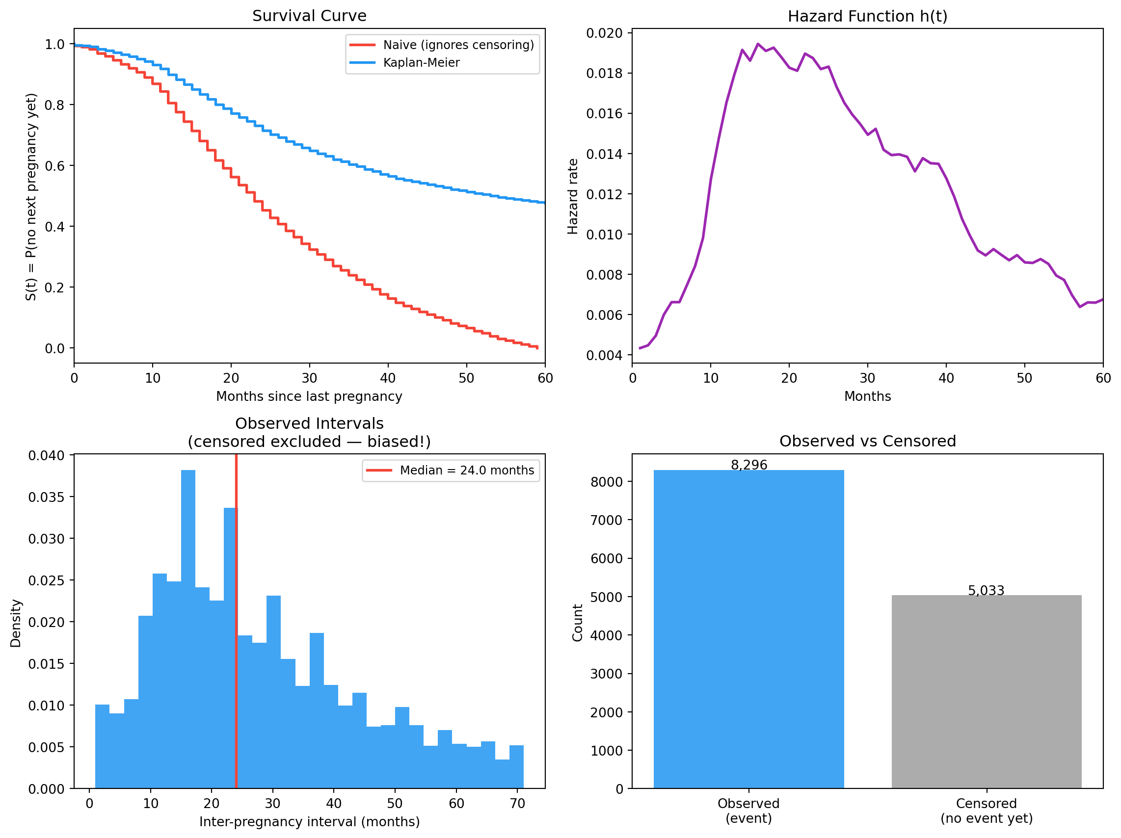
Naive vs KM survival, the hazard function, the observed-interval distribution, and the observed/censored split.

27.9 Cohort effects

Different generations may have different survival curves. Women born in 1960 vs 1975 may have different inter-pregnancy intervals (different fertility patterns, economics, etc.). Computing separate KM curves for cohorts and comparing reveals these shifts.

27.10 Expected remaining lifetime

Given that you’ve survived to time t, how much longer do you expect to wait?

E[T - t \mid T > t] \;=\; \frac{\int_t^\infty S(u)\, du}{S(t)}

This answers a different question than the unconditional mean — and the answer differs.

27.11 Exercises

Compute inter-pregnancy intervals using NSFG.
Identify which women are censored (only one pregnancy recorded).
Implement the Kaplan-Meier estimator from scratch.
Plot the KM survival curve.
Compare KM curves for women in different age cohorts.

27.12 Glossary

survival analysis — methods for time-to-event data with possible censoring.

survival function S(t) — probability of no event before time t.

hazard function h(t) — instantaneous event rate at time t, given survival to t.

censored observation — event has not (yet) occurred; we know T > t but not T.

right censoring — the most common type: event hasn’t happened by end of observation.

Kaplan–Meier — nonparametric estimate of survival that handles censoring.

at risk — observations that have not yet had the event and have not been censored.

cohort effect — survival differences between groups defined by birth year.