Every day you make decisions under uncertainty. Will the bridge hold? Is this email spam? Will the drug work? Will it rain? You cannot know the answer with certainty — but you are not helpless. You can reason carefully about the likelihood of different outcomes, and that reasoning is what probability theory formalises.
NoteA conversation at a hospital
Relative: Nurse, what is the probability the drug will work?
Nurse: I hope it works — we’ll know tomorrow.
Relative: Yes, but what is the probability it will?
Nurse: Each case is different. We have to wait.
Relative: Out of a hundred patients treated under similar conditions, how many times would you expect it to work?
Nurse:(somewhat annoyed) I told you, every person is different.
Relative: Then if you had to bet whether it will work — which side would you take?
Nurse:(cheering up briefly) I’d bet it will work.
Relative: Would you accept losing $2 if it doesn’t, and gaining $1 if it does?
Nurse:(exasperated) What a sick thought! You are wasting my time!
This exchange captures something important. The relative tried two completely different definitions of probability:
“Out of a hundred patients…” — probability as a long-run frequency.
“Which side of the bet would you take?” — probability as a degree of belief that can be elicited from someone’s willingness to bet.
The nurse refused both. She wasn’t being unreasonable — she was sensing that this particular patient is unique. That tension — between the universal (population-level) and the particular (this-case) — is the central problem the rest of this chapter addresses.
Probability is not just an academic tool. It is the language of uncertainty — used in weather forecasting, medical diagnosis, engineering reliability, financial risk, and machine learning.
3.2 A short history
What’s surprising is that probability is young. Mathematicians had been doing calculus and geometry for centuries before anyone took randomness seriously enough to write equations about it. The story of how probability became a real subject is short, dramatic, and full of gamblers, monks, astronomers, and one telephone engineer who quietly changed the world.
Click any name to read more.
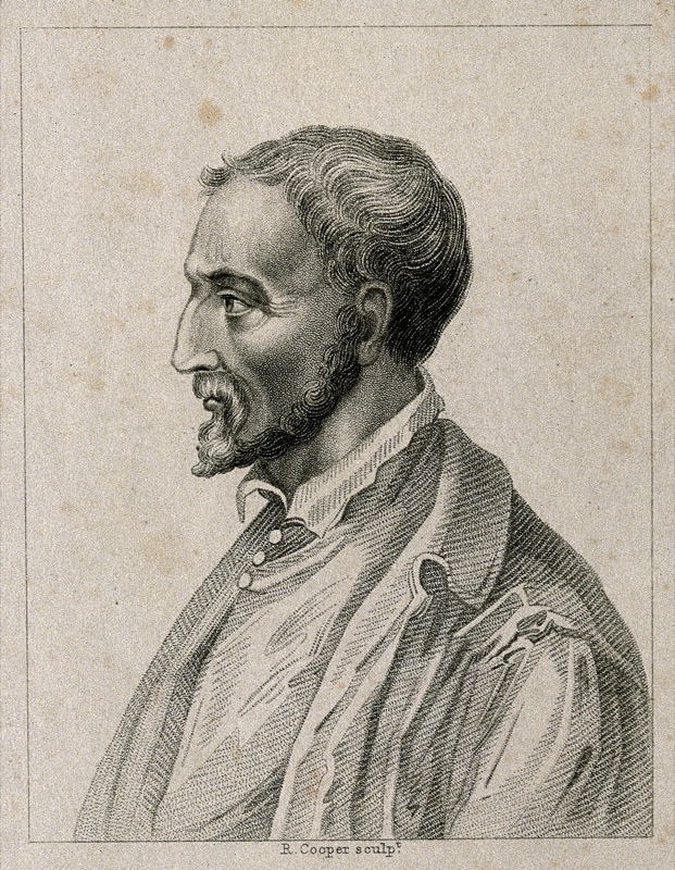
Tip▶ Gerolamo Cardano (1501–1576) — the gambling doctor
A 16th-century Italian physician, mathematician, and chronic gambler. Cardano wrote Liber de Ludo Aleae (“Book on Games of Chance”) around 1560 — the first known systematic treatment of probability. He worked out odds for dice, cards, and backgammon, and even discussed how to detect cheating.
Embarrassed by the subject’s disreputable connections, he kept the manuscript private. It wasn’t published until 1663 — almost 90 years after his death. Cardano’s instincts were correct, but the field had to be re-discovered by mathematicians who took it more seriously.
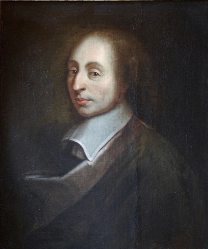
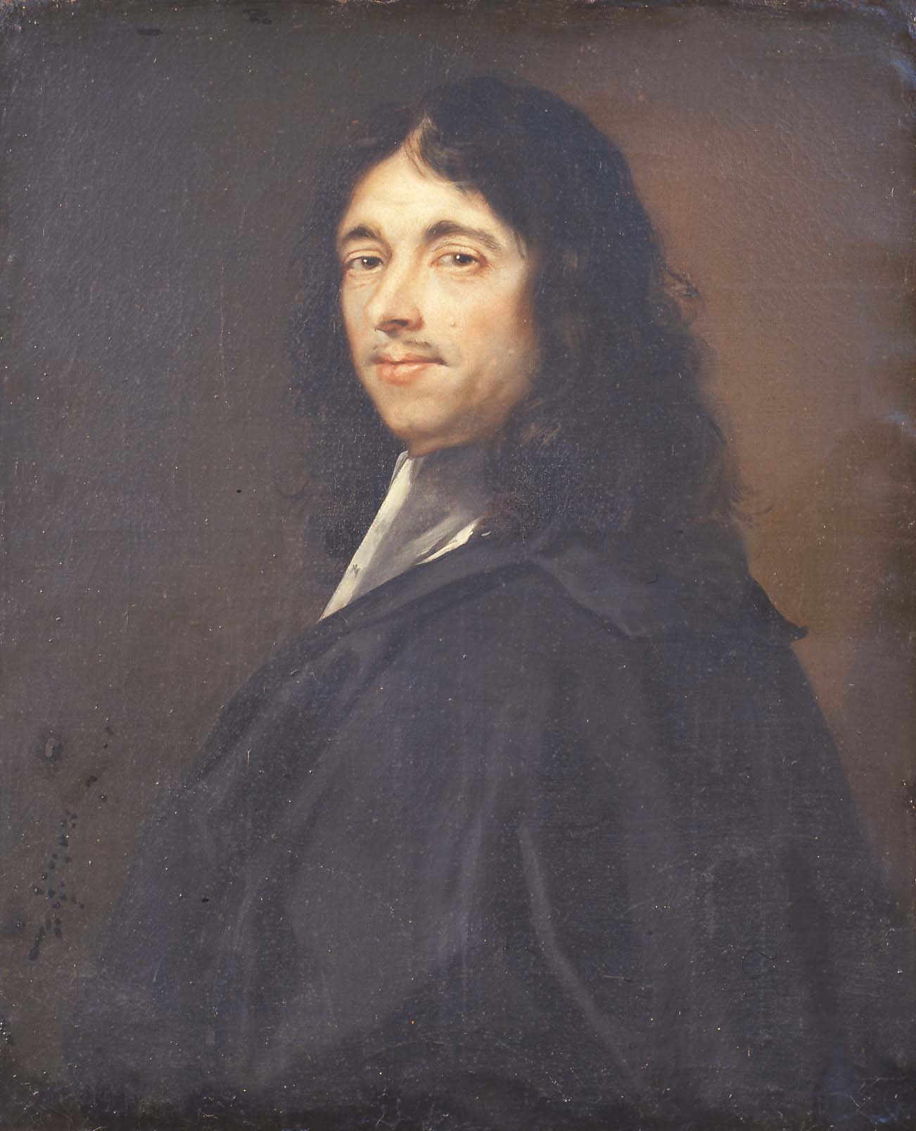
Tip▶ Blaise Pascal & Pierre de Fermat (1654) — letters that founded a field
Blaise Pascal (1623–1662)
Pierre de Fermat (1601–1665)
A French nobleman named the Chevalier de Méré asked Pascal a question about a dice game: if a game has to stop early, how should the pot be divided fairly between the players?
Pascal didn’t know. He wrote to Fermat in 1654, and the two exchanged a series of letters working out the answer. In doing so they invented — almost by accident — the foundations of probability theory: expected value, the multiplication rule, the structure of compound events. Six letters. The field begins here.
The problem they solved is still called the problem of points, and their solution is still the right one.
Pascal portrait: copy of François Quesnel (1691), Palace of Versailles (Wikimedia, CC BY 3.0). Fermat portrait: oil on canvas by Rolland Lefebvre, c. 1650 (Wikimedia, public domain).
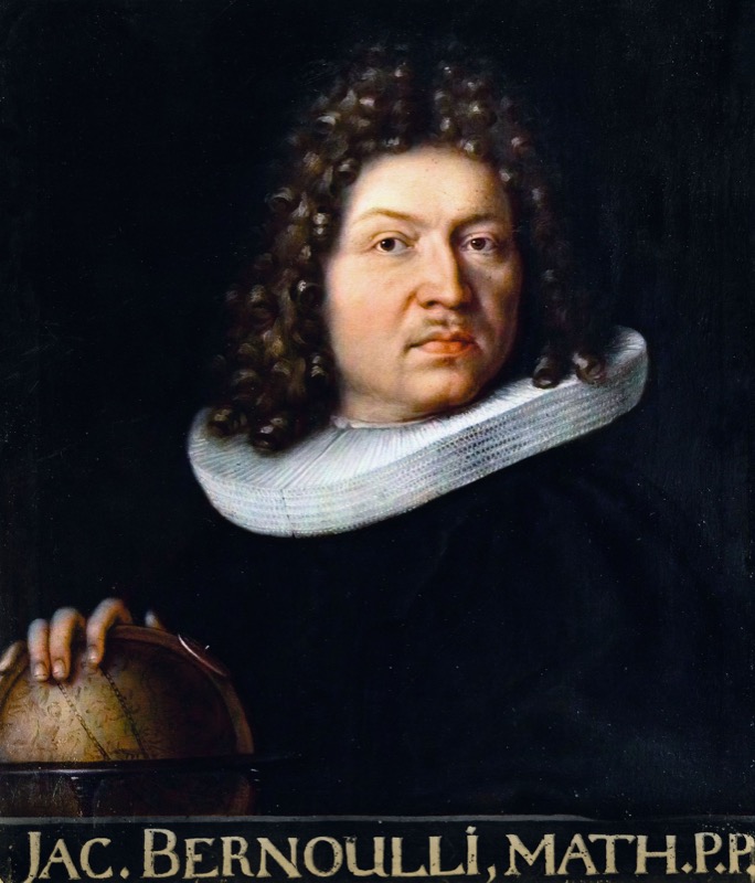
Tip▶ Jacob Bernoulli (1654–1705) — the law of large numbers
Twenty years after Pascal and Fermat, the Swiss mathematician Jacob Bernoulli took up the question: if I flip a coin enough times, does the fraction of heads actually converge to its true probability?
Yes — and he proved it. His Law of Large Numbers (published posthumously in 1713 in Ars Conjectandi) is the bridge between frequencies you can measure and probabilities you cannot. It turns probability from a calculator’s curiosity into a science: the empirical world can be used to estimate the unseen.
Every time you compute an average, you are leaning on his theorem.
Portrait by his brother Niklaus Bernoulli, c. 1687 (Wikimedia, public domain).
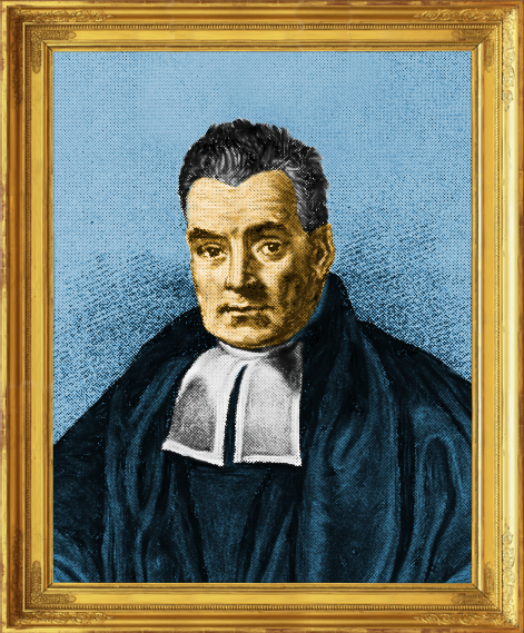
Tip▶ Thomas Bayes (1701–1761) — the rule that runs modern AI
An English Presbyterian minister and amateur mathematician, Bayes wrote a paper on inverse probability — given an observed effect, what was the likely cause? — and never published it. After his death, his friend Richard Price found it in his papers and submitted it to the Royal Society in 1763.
For 200 years it was a curiosity. Then statisticians, and later machine learning researchers, noticed something: Bayes’ rule is the mathematics of learning from evidence. Every spam filter, every medical diagnostic system, every Bayesian neural network is a child of this short paper by a country minister who didn’t think it worth printing.
We’ll meet his rule formally a few chapters from now. It deserves the build-up.
The only commonly-circulated portrait traditionally identified as Thomas Bayes — its authenticity is disputed by historians (no verified likeness of Bayes survives). Colorized version by Mark Riehl (Wikimedia, CC BY-SA 4.0).
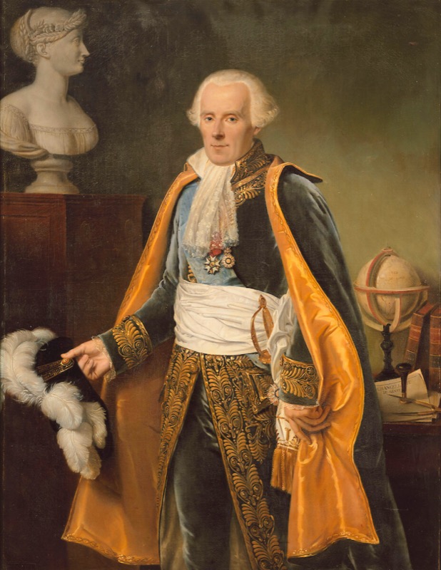
Tip▶ Pierre-Simon Laplace (1749–1827) — the great consolidator
If Bayes was the seed, Laplace was the gardener. The French polymath generalized Bayes’ rule, applied probability to astronomy, geodesy, demographics, and law, and wrote Théorie Analytique des Probabilités (1812) — the first comprehensive textbook of the subject.
Laplace took probability seriously as a science. He used it to weigh witness testimony in court cases, to estimate the population of France from a sample, to argue that the solar system was stable. After Laplace, no one could dismiss probability as gambler’s mathematics again.
A famous quip attributed to him: “It is remarkable that a science which began with the consideration of games of chance should have become the most important object of human knowledge.”
Portrait by Jean-Baptiste Paulin Guérin, 1838, Palace of Versailles (Wikimedia, public domain).
Tip▶ Andrey Kolmogorov (1903–1987) — the axioms
Until 1933, probability was a working subject without a formal foundation. Different mathematicians used different definitions; the field had paradoxes nobody could agree how to resolve.
Then a 30-year-old Soviet mathematician named Andrey Kolmogorov published Grundbegriffe der Wahrscheinlichkeitsrechnung — a slim monograph in which he proposed that probability theory should be built on three simple axioms (the ones we’ll meet later in this chapter) plus measure theory.
Within a decade, the entire field had reorganised around his framework. Every textbook written since 1933 — including this one — uses Kolmogorov’s axioms. The formal foundation of probability is younger than your grandparents.
Tip▶ Claude Shannon (1916–2001) — the bridge to machine learning
A telephone engineer at Bell Labs, Shannon noticed something nobody else had: information itself can be measured probabilistically. His 1948 paper A Mathematical Theory of Communication introduced entropy (H = -\sum p_i \log p_i), the bit, and the channel capacity theorem.
Shannon’s work is why you can make a phone call, store data on a hard drive, compress a file, or train a neural network. Every loss function in deep learning that has the word cross-entropy in it is a tribute to him. He also liked to ride a unicycle through the Bell Labs corridors while juggling.
If you take only one name from this list with you, take Shannon. He is the reason probability and computation became inseparable.
Photos of Shannon are still under copyright. The Bell Labs and MIT Museum archives hold the famous portraits.
That’s roughly four centuries of work, ending 75 years ago. The subject is still young. With that history in your pocket, let’s see what probability actually says.
3.3 The two-stage framework
There are really two stages to applying probability to a real problem:
TipTwo Stages of Probabilistic Modelling
Stage 1 — Modelling (art). Decide on a sample space and a probability law. There are no rigid rules here. Reasonable people will disagree about which model fits.
Stage 2 — Analysis (science). Once the model is fixed, calculate probabilities. There is exactly one right answer; only your skill determines whether you find it.
Most “paradoxes” in probability are arguments about Stage 1 disguised as arguments about Stage 2. When two clever people get different answers to the same problem, they almost never disagree about the math — they disagree about which model is right.
The discipline of this chapter is to make Stage 1 explicit before calculating anything.
3.3.1 Why the Model Matters: The Two-Child Puzzle
Abstract claims about “Stage 1 vs Stage 2” only land once you’ve watched two clever people disagree about a real problem. Here’s one. It’s short, it’s famous, and it has stumped working mathematicians.
You meet a stranger at a party. She tells you, “I have two children, and at least one of them is a boy.” What is the probability that both of her children are boys?
Take a moment. Write down your answer before reading on. Most people say 1/2 — “the other child is either a boy or a girl, those are equally likely, so 1/2.” Others, after some thought, say 1/3. A few say “it depends” and look smug.
Here’s the thing: both 1/3 and 1/2 can be defended, and the disagreement is entirely about Stage 1 — what sample space should we use? Once a sample space is fixed, every reasonable person gets the same number out. Let’s see this happen.
Model A — “boy first, girl second” is a different family from “girl first, boy second”. Birth order matters; the four equally likely families are:
The stranger told us “at least one is a boy”, so we eliminate GG. Three families remain — BB, BG, GB — and all three are still equally likely (we haven’t been given any reason to prefer one over the others). Of those three, only BB has two boys. So P(\text{both boys}) = 1/3.
Model B — we already met one of the children, and he was a boy. Maybe she said it because the boy was standing next to her. In that case, the information isn’t “at least one is a boy” — it’s “this specific child is a boy”. The other child is then independent of the one we met, and is a boy or a girl with equal probability. So P(\text{both boys}) = 1/2.
So what actually changed? The two models aren’t disagreeing about the rules of probability — they’re reasoning over different sample spaces.
Model A samples families. Start with the four equally likely families \{\text{BB}, \text{BG}, \text{GB}, \text{GG}\}, filter out the ones with no boy. Three families survive; only one is BB.
Model B samples a specific child and asks about their sibling. Once one child has been identified as a boy, BG and GB are no longer two distinct outcomes — they collapse into “this boy plus one unknown sibling”, and the sibling is a fresh coin flip.
The verbal sentence “at least one is a boy” is the same in both stories, but it was generated by two different experiments. The sample space follows the experiment, not the sentence.
Two models, two different answers. Nobody has done arithmetic yet. The argument is happening at Stage 1.
We can confirm Model A’s answer by simulation — pick the model and the math falls out.
# Model A: simulate many two-child families. Each child is independently# B or G with probability 1/2. Among families with AT LEAST ONE boy, what# fraction have TWO boys?import numpy as nprng = np.random.default_rng(seed=0)n_families =200_000child_1 = rng.integers(0, 2, size=n_families) # 1 = boy, 0 = girlchild_2 = rng.integers(0, 2, size=n_families)at_least_one_boy = (child_1 ==1) | (child_2 ==1)both_boys = (child_1 ==1) & (child_2 ==1)# Conditional frequency: among families with at least one boy,# the fraction that have two boys.p_model_A = both_boys.sum() / at_least_one_boy.sum()print(f"Model A simulation: P(both boys | at least one boy) ≈ {p_model_A:.4f}")print(f"Theoretical answer: 1/3 ≈ {1/3:.4f}")
Model A simulation: P(both boys | at least one boy) ≈ 0.3324
Theoretical answer: 1/3 ≈ 0.3333
# Model B: simulate the same families, but now we 'meet' a uniformly random# child from each family. Condition on the child we met being a boy, and ask# whether the OTHER child is also a boy.# Pick a random child to 'meet' from each family (0 = first, 1 = second)which_met = rng.integers(0, 2, size=n_families)met_child = np.where(which_met ==0, child_1, child_2)other_child = np.where(which_met ==0, child_2, child_1)met_a_boy = (met_child ==1)other_is_boy = (other_child ==1)p_model_B = other_is_boy[met_a_boy].mean()print(f"Model B simulation: P(other child is boy | met a boy) ≈ {p_model_B:.4f}")print(f"Theoretical answer: 1/2 ≈ {1/2:.4f}")
Model B simulation: P(other child is boy | met a boy) ≈ 0.5004
Theoretical answer: 1/2 ≈ 0.5000
The simulations agree with the theory for whichever model you chose. The math is not in dispute. The model is.
TipThe lesson
When someone claims a probability problem has a “right” answer and a “wrong” answer, your first job is not to do the calculation. It’s to ask: what sample space are you using, and why? Almost every probability paradox you’ll meet — Monty Hall, the Sleeping Beauty problem, the boy-girl paradox above, the envelope paradox — is a Stage 1 disagreement wearing a Stage 2 costume. The math is fine. The modelling is what people are actually arguing about.
Throughout this book, whenever we set up a problem, we’ll spell out \Omega first. It’s a habit worth building.
Note▶ Two-stage framework in action — web click model
A tech company wants to model whether a user clicks an ad. Three data scientists each propose a model:
Model A — Simple.\Omega = \{\text{Click},\ \text{No Click}\}, P(\text{Click}) = 0.15 (historical average). Justification: Easy to use, captures overall rate.
Model B — Time-aware.\Omega = \{\text{Click},\ \text{No Click}\} \times \{\text{Morning},\ \text{Afternoon},\ \text{Evening}\}, with different click probabilities for each time slot. Justification: More accurate; accounts for daily patterns.
Model C — Full ML model. Sample space includes user demographics, device type, browsing history. Probability law comes from a trained model. Justification: Highest accuracy; highest cost.
Who is right? All three are valid — they satisfy the axioms. The choice depends on what questions need answering, computational resources, and required accuracy. This is Stage 1: reasonable people can disagree.
Once Model A is fixed, Stage 2 has a unique answer. Q: “What’s the probability of exactly 3 clicks from 10 users?”P(X = 3) = \binom{10}{3}(0.15)^3(0.85)^7 \approx 0.130 No ambiguity — the model determines the answer exactly.
Note▶ The Birthday “Paradox” — a Stage 1 disagreement
The claim: “In a room of 30 people, what’s the probability two share a birthday?”
These are different questions, not different calculations of the same thing. The verbal sentence “two share a birthday” was understood differently by each analyst.
Resolution. Once both analysts explicitly write down:
The sample space \Omega
The exact event of interest
Their assumptions
— the apparent paradox vanishes. There is no paradox, only ambiguity at Stage 1.
import numpy as nprng = np.random.default_rng(99)n_sim =200_000n_people =30# Analyst 1: probability some pair share a birthdaybirthdays = rng.integers(0, 365, size=(n_sim, n_people))has_shared = np.array([len(set(row)) < n_people for row in birthdays])print(f"Analyst 1 (any shared birthday): {has_shared.mean():.4f} (theory ≈ 0.7063)")# Analyst 2: probability someone shares MY birthday (day 0)my_birthday =0has_match = np.any(birthdays[:, 1:] == my_birthday, axis=1)print(f"Analyst 2 (matches my birthday): {has_match.mean():.4f} (theory ≈ 0.0765)")
A probabilistic model is a mathematical description of an uncertain situation. Every probabilistic model is built in exactly two steps:
Describe the sample space — list all possible outcomes.
Assign a probability law — specify how likely each outcome (or collection of outcomes) is.
This two-step structure is the backbone of everything that follows. But before we build the machinery, there is a prior question worth settling: what does the number P(A) = 0.7 actually mean?
3.5 Interpretations of Probability
The probability axioms (which we will meet in Section 4) tell us the rules the numbers must obey. They say nothing about what the numbers mean. There are two schools of thought.
3.5.1 The Frequentist View: Probability as Long-Run Frequency
The probability of an event is the long-run frequency with which it happens if you could repeat the experiment infinitely many times.
This is intuitive for repeatable things. “This coin lands heads with probability 0.5” means: if you flip it enough times, the fraction landing heads converges to 0.5.
Notice three things in the animation:
The first 10 flips are all over the place. The fraction is 0, or 1, or 0.6, depending on what came up. Frequency is not probability when the sample is small.
By the time we have 100+ flips, the fraction is close to 0.5 and stays close. That’s frequency converging to probability.
It never settles exactly. It zigzags around 0.5 forever, the zigzag getting smaller as n grows.
The frequentist says: “the probability of heads is 0.5” is a statement about that limit. The behaviour you see in the animation — the convergence — is the empirical content of the claim.
Note▶ Show the math — The Law of Large Numbers, briefly
If X_1, X_2, \ldots are independent flips of the same coin (each X_i = 1 with probability p, 0 otherwise), the sample mean \bar{X}_n = \frac{1}{n}\sum_{i=1}^n X_i satisfies \bar{X}_n \to p as n \to \infty. Both the weak law (convergence in probability) and the strong law (almost-sure convergence) make this rigorous. A full proof uses Chebyshev’s inequality — we return to it in the limit theorems chapter.
3.5.2 The Subjective View: Probability as Degree of Belief
The probability of an event, for a given person at a given time, is revealed by the bets they are willing to take on it.
Look at the opening dialogue again. The relative offered this bet:
Drug works → nurse gains $1
Drug does not work → nurse loses $2
Let p be the nurse’s belief that the drug works. Her expected profit is p \cdot 1 + (1-p) \cdot (-2) = 3p - 2. A rational person only accepts a bet with non-negative expected profit:
3p - 2 \ge 0 \implies p \ge \tfrac{2}{3}
By accepting, the nurse reveals she believes the drug works with probability at least 67%. The general rule: if the bet pays $W when you win and costs $L when you lose, accept only if:
The subjectivist says:
NoteDeriving the threshold p \ge \frac{L}{W+L}
A rational person accepts a bet only if its expected profit is non-negative. For a bet that pays $W on a win and costs $L on a loss:
E[\text{profit}] = p \cdot W + (1 - p) \cdot (-L) \ge 0
Expand and collect:
pW - L + pL \ge 0 \implies p(W + L) \ge L \implies p \ge \frac{L}{W + L}
Check with the nurse’s bet (W = 1, L = 2): p \ge \frac{2}{1 + 2} = \frac{2}{3} \approx 67\% \checkmark
Intuition: the threshold is the fraction of the total stake that you stand to lose. The bigger the loss relative to the win, the more confident you need to be before it is worth taking the bet.
Tip▶ Historical note
Christiaan Huygens (1657) introduced expected value in De Ratiociniis in Ludo Aleae — the formula E[\text{profit}] = pW - (1-p)L comes from his definition.
Jakob Bernoulli (1713) proved the Law of Large Numbers, justifying the rule across many bets.
Daniel Bernoulli (1738) pointed out in the St. Petersburg paradox that real people maximise expected utility, not expected money — losing $2 hurts more than gaining $2 helps, so in practice you need higher confidence than the break-even threshold.
This view works for one-shot events, historical claims, personal beliefs — anywhere repetition is impossible.
Where it runs out of road: different people can have different priors and so different probabilities for the same event. Frequentists find this disturbing; subjectivists say it is just honest.
3.5.3 One Math, Two Meanings
Both views obey the same axioms — the mathematics is identical. We will use whichever interpretation fits the problem. For coin flips and dice, frequentist intuition is sharper. For “how confident is this classifier?”, subjective intuition is sharper.
A useful mental model for how the two fields relate:
flowchart LR
    RW["🌍 Real World"]
    PM["📐 Probabilistic Model"]
    R["📊 Results"]

    RW -->|"Statistics: inference"| PM
    PM -->|"Probability: analysis"| R
    R  -->|"Predictions / decisions"| RW
flowchart LR
    RW["🌍 Real World"]
    PM["📐 Probabilistic Model"]
    R["📊 Results"]

    RW -->|"Statistics: inference"| PM
    PM -->|"Probability: analysis"| R
    R  -->|"Predictions / decisions"| RW
3.6 The Sample Space
3.6.1 Definition
ImportantSample Space
The sample space\Omega is the set of all possible outcomes of an experiment. Each element of \Omega is called an outcome.
For \Omega to be valid, the outcomes must satisfy two properties:
Mutually exclusive: At the end of the experiment, exactly one outcome occurs. No two distinct outcomes can both occur.
Collectively exhaustive: Together, the outcomes cover all possibilities. No matter what happens, one outcome from \Omega must occur.
Summary: At the end of the experiment, you can point to one — and exactly one — outcome in \Omega.
3.6.2 The Granularity Principle
How much detail should a sample space contain? The answer depends on the questions you want to answer.
Option B is not wrong — it is still mutually exclusive and collectively exhaustive. But it includes weather information that is irrelevant to the coin. Option A is the right choice unless you believe weather affects the coin’s outcome.
TipThe Granularity Principle
Include details that are relevant to the questions you want to answer. Exclude details that are irrelevant — they only add complexity without improving the model.
The right level of detail is not always obvious. Consider a clinical trial:
Too little detail: \Omega = \{\text{drug works},\ \text{drug doesn't work}\} — cannot capture how well it works.
Too much detail: \Omega = \{\text{every molecular interaction in every patient}\} — impossible to work with.
import pandas as pdimport numpy as np# Enumerate all 36 outcomesoutcomes = [(d1, d2) for d1 inrange(1, 7) for d2 inrange(1, 7)]print(f"Total outcomes: {len(outcomes)}")print("First few:", outcomes[:6])
Total outcomes: 36
First few: [(1, 1), (1, 2), (1, 3), (1, 4), (1, 5), (1, 6)]
The same experiment can be modelled with very different sample spaces depending on how much detail we keep. Let’s compare three of them.
What does each one let us ask?
Sample space (A) — sums only. Good for “what’s the probability the sum is 7?”. But it cannot answer “was the first die a 6?” — that information has been thrown away.
Sample space (C) — pairs + colour + rotation angle. Can answer everything, but adds no value for typical dice questions.
Sample space (B) — ordered pairs. Can answer every question we actually care about and nothing more. This is the right level of detail.
TipChoosing the sample space is part of modelling
There is no “the” sample space for an experiment. There is the sample space you choose for the questions you want to answer. This is the clearest example of Stage 1 (modelling = art) at work.
WarningWhy mutual exclusivity matters
Compare these two attempted sample spaces for a single die roll:
\Omega_{\text{good}} = \{1, 2, 3, 4, 5, 6\} ✓
\Omega_{\text{bad}} = \{\text{"1 or 3"}, \text{"1 or 4"}, 2, 3, 5, 6\} ✗
The second one is broken. If you roll a 1, which outcome occurred — “1 or 3” or “1 or 4”? The outcomes overlap (both contain a 1), so the result of the experiment isn’t uniquely defined. Probability calculations break immediately: the axioms assume disjointness when adding.
A working sample space must let you point at exactly one outcome after the experiment runs. No ambiguity.
Tip▶ Sample space design: Two coin-flipping games
This example from Bertsekas & Tsitsiklis (§1.1) shows why the right sample space depends on the questions you want to answer — even when the underlying experiment is identical.
Setup. Ten successive fair coin tosses. Two games are played:
Game 1. You earn $1 for each heads.
Game 2. You earn $1 per toss until the first heads, then $2 per toss until the second heads, then $4 per toss, doubling the rate each time a heads appears.
The underlying sample space (all sequences of length 10): \Omega = \{\text{all sequences of H and T of length 10}\}, \quad |\Omega| = 2^{10} = 1024
Game 1 — simplified space is enough. Only the total count of heads determines the payout, so we can use: \Omega_1 = \{0, 1, 2, \ldots, 10\} All 11 sequences with the same head-count give the same $-amount, so collapsing them loses nothing. This simplification makes analysis tractable.
Game 2 — must use the full space. The positions of heads matter. Compare two sequences with exactly 4 heads:
Toss
HHTTTHTHTT
HTHTTTTHTH
1
H → $1
H → $1
2
H → $2
T → $2
3
T → $4
H → $2
4
T → $4
T → $4
5
T → $4
T → $4
6
H → $4
T → $4
7
T → $8
T → $4
8
H → $8
H → $4
9
T → $16
T → $8
10
T → $16
H → $8
Total
$67
$41
Same number of heads, different positions → different payouts. We must use all 1024 sequences for Game 2.
Key insight. Both games share the same physical experiment, but the right sample space is different:
Game
Sample space
Why
Game 1
\{0,1,\ldots,10\} (11 outcomes)
Order doesn’t matter
Game 2
All 1024 sequences
Order changes the payout
Choosing the right level of detail is not about being more careful — it’s about matching the sample space to the questions you need to answer.
3.6.4 Continuous Sample Spaces
Some experiments have outcomes that take any value in a continuous range — a waiting time, a voltage, an angle, a position. The sample space is no longer a list but a continuous region.
Example: Spinning a game-show wheel with numbers from 0 to 1. The pointer can land anywhere — the sample space is:
\Omega = [0, 1]
There are uncountably many possible outcomes. You cannot list them. This is a continuous sample space.
Example: Two arrival times — Romeo and Juliet each arrive at a random time in [0,1] hour. The sample space is the unit square:
\Omega = \{(x, y) \mid 0 \le x \le 1,\ 0 \le y \le 1\}
There are uncountably many pairs (x, y) — again, you cannot list them.
For now we are only describing what the sample space looks like. How to assign probabilities to regions of a continuous space requires the axioms, which we introduce in the next section. Once we have those tools, we return to both examples and compute probabilities properly.
3.7 Probability Laws and Axioms
3.7.1 Motivation
We need a rule that assigns a number P(A) to every event A, capturing how likely it is. What properties should such a rule have?
Think about it intuitively:
A likelihood below zero makes no sense — so probabilities must be non-negative.
Something must happen — so the total probability of the entire sample space must be 1.
If two events cannot both occur (disjoint events), the probability of either one happening is the sum of their individual probabilities.
These three intuitions are the axioms — the minimum set of rules needed for a consistent and useful theory of probability.
ImportantThe Kolmogorov Axioms
A probability lawP is a function that assigns a number P(A) to every event A \subseteq \Omega, satisfying:
(A1) Non-negativity.P(A) \ge 0 for every event A.
(A2) Normalization.P(\Omega) = 1.
(A3) Additivity. If A and B are disjoint (A \cap B = \emptyset), then P(A \cup B) = P(A) + P(B).
Think of probability as mass. Imagine spreading 1 kilogram of mass over the sample space. P(A) is the mass sitting on top of region A. Non-negativity says mass can’t be negative. Normalization says the total mass is 1 kg. Additivity says non-overlapping regions just add their masses.
Three axioms. That is the entire foundation. Everything else in probability — every formula, theorem, and proof — follows from these three.
Let’s verify them on our two-dice example.
import numpy as np# Two-dice sample space: all 36 ordered pairsoutcomes = [(d1, d2) for d1 inrange(1, 7) for d2 inrange(1, 7)]omega =set(outcomes)# For fair dice, each of the 36 outcomes has probability 1/36.def P(event):returnlen(event) /36A = {(d1, d2) for d1, d2 in omega if d1 + d2 ==7} # sum is 7# (A1) Non-negativityprint(f"(A1) P(A) = {P(A):.4f} ≥ 0 ✓")# (A2) Normalizationprint(f"(A2) P(Ω) = {P(omega)} = 1 ✓")# (A3) Additivity — pick two disjoint eventsE = {(d1, d2) for d1, d2 in omega if d1 + d2 ==7}F = {(d1, d2) for d1, d2 in omega if d1 + d2 ==11}print(f" E ∩ F = {E & F} (disjoint ✓)")print(f" P(E) + P(F) = {P(E):.4f} + {P(F):.4f} = {P(E) + P(F):.4f}")print(f" P(E ∪ F) = {P(E | F):.4f}")print(f" Equal ✓")
The additivity axiom above handles two disjoint events. But many experiments have infinitely many possible stages. Consider tossing a coin until the first heads appears — the number of tosses could be 1, 2, 3, … with no bound. The events “first heads on toss n” are mutually exclusive for different n, and together they cover all possibilities. We need:
If A_1, A_2, A_3, \ldots is an infinite sequence of pairwise disjoint events, then: P\!\left(\bigcup_{i=1}^{\infty} A_i\right) = \sum_{i=1}^{\infty} P(A_i)
The word sequence here is critical — we need the events to be arrangeable in a list (countably many). This works for coin tosses, dice rolls, integers. It does not apply to uncountable collections like every individual point in [0,1] — we will see why shortly.
3.8 Derived Properties of Probability
From just the three axioms, we can derive every useful property of probability:
Note▶ Show the math — Useful consequences of the axioms
1. P(\emptyset) = 0.
Proof.\Omega = \Omega \cup \emptyset and these are disjoint, so by (A3): P(\Omega) = P(\Omega) + P(\emptyset), which gives P(\emptyset) = 0. \blacksquare
2. Complement rule: P(A^c) = 1 - P(A).
Proof.A and A^c are disjoint and A \cup A^c = \Omega. By (A3): P(A) + P(A^c) = P(\Omega) = 1. \blacksquare
3. Upper bound: P(A) \le 1.
Proof. From (2), P(A) = 1 - P(A^c) \le 1 since P(A^c) \ge 0 by (A1). \blacksquare
4. Monotonicity: if A \subseteq B, then P(A) \le P(B).
Proof. Write B as a disjoint union: B = A \cup (B \cap A^c). By (A3): P(B) = P(A) + P(B \cap A^c) \ge P(A). \blacksquare
Proof. Decompose A \cup B into three disjoint pieces: A \cup B = (A \cap B^c) \;\sqcup\; (A^c \cap B) \;\sqcup\; (A \cap B). Apply (A3) and rearrange. \blacksquare
6. Union bound (Boole’s inequality):P(A \cup B) \le P(A) + P(B), \qquad P\!\left(\bigcup_i A_i\right) \le \sum_i P(A_i).
Proof. For two events, this is (5) plus P(A \cap B) \ge 0. \blacksquare
The union bound looks weak — it just throws away the intersection — but it’s used constantly in machine learning theory because it requires no assumptions about how the events relate to each other.
# Verify all properties numerically on the dice exampleomega_set =set(outcomes)n =len(omega_set) # 36def P_check(event):returnlen(event) / nA_ev = {(i, j) for i, j in omega_set if i ==1} # first die = 1B_ev = {(i, j) for i, j in omega_set if i + j >=10} # sum >= 10print(f"P(A) = {P_check(A_ev):.4f}")print(f"P(B) = {P_check(B_ev):.4f}")print(f"P(A^c) = {P_check(omega_set - A_ev):.4f} (should be 1 - P(A) = {1- P_check(A_ev):.4f})")print(f"P(A ∩ B) = {P_check(A_ev & B_ev):.4f}")print(f"P(A ∪ B) = {P_check(A_ev | B_ev):.4f}")print(f"P(A) + P(B) - P(A ∩ B) = {P_check(A_ev) + P_check(B_ev) - P_check(A_ev & B_ev):.4f} (inclusion-exclusion ✓)")
P(A) = 0.1667
P(B) = 0.1667
P(A^c) = 0.8333  (should be 1 - P(A) = 0.8333)
P(A ∩ B) = 0.0000
P(A ∪ B) = 0.3333
P(A) + P(B) - P(A ∩ B) = 0.3333  (inclusion-exclusion ✓)
3.9 Events
3.9.1 Events on a Discrete Sample Space
An event is just a subset of \Omega. Some examples for our two dice:
omega =set(outcomes)A = {(d1, d2) for d1, d2 in omega if d1 + d2 ==7} # sum is 7B = {(d1, d2) for d1, d2 in omega if d1 == d2} # doublesC = {(d1, d2) for d1, d2 in omega if d1 ==6} # first die is 6D = {(d1, d2) for d1, d2 in omega if d1 + d2 >=10} # sum ≥ 10print(f"A = sum is 7 ({len(A)} outcomes): {sorted(A)}")print(f"B = doubles ({len(B)} outcomes): {sorted(B)}")print(f"C = first die is 6 ({len(C)} outcomes): {sorted(C)}")print(f"D = sum ≥ 10 ({len(D)} outcomes): {sorted(D)}")
A = sum is 7        (6 outcomes): [(1, 6), (2, 5), (3, 4), (4, 3), (5, 2), (6, 1)]
B = doubles         (6 outcomes): [(1, 1), (2, 2), (3, 3), (4, 4), (5, 5), (6, 6)]
C = first die is 6  (6 outcomes): [(6, 1), (6, 2), (6, 3), (6, 4), (6, 5), (6, 6)]
D = sum ≥ 10        (6 outcomes): [(4, 6), (5, 5), (5, 6), (6, 4), (6, 5), (6, 6)]
Because events are sets, you can combine them with set operations. Combining events gives you new events:
# Sum is 7 OR doublesA_or_B = A | B # set union → "A or B"# Sum is 7 AND first die is 6 → exactly one roll: (6, 1)A_and_C = A & C # set intersection → "A and C"# Sum is 7 but NOT doublesA_not_B = A - B # set difference → "A but not B"# Sum is 7 AND doubles → impossible (no double sums to 7), so empty setA_and_B = A & Bprint(f"A ∪ B ('sum is 7 OR doubles'): {len(A_or_B)} outcomes")print(f"A ∩ C ('sum is 7 AND first die is 6'): {len(A_and_C)} outcomes → {A_and_C}")print(f"A - B ('sum is 7 but not doubles'): {len(A_not_B)} outcomes")print(f"A ∩ B ('sum is 7 AND doubles'): {len(A_and_B)} outcomes → {A_and_B} (empty set ∅)")
A ∪ B   ('sum is 7 OR doubles'):           12 outcomes
A ∩ C   ('sum is 7 AND first die is 6'):   1 outcomes  →  {(6, 1)}
A - B   ('sum is 7 but not doubles'):      6 outcomes
A ∩ B   ('sum is 7 AND doubles'):          0 outcomes  →  set()  (empty set ∅)
A few things to notice in the output:
A ∩ C gives the single roll (6, 1) — the first die is 6 and the sum is 7. So this intersection is not empty.
A ∩ Bis empty, because no double (k, k) sums to 7 (we’d need 2k = 7, but k has to be a whole number from 1 to 6). When two events cannot happen together, their intersection is the empty set \emptyset, and we say they are disjoint or mutually exclusive.
That’s the entire grammar. Set union for “or”, set intersection for “and”, set complement for “not”. Probability theory inherits its grammar from set theory.
Note▶ Show the math — Set algebra and De Morgan’s laws
For any events A, B, C \subseteq \Omega, the following identities hold and are used constantly:
Commutative.A \cup B = B \cup A, \;\; A \cap B = B \cap A.
Associative.(A \cup B) \cup C = A \cup (B \cup C), \;\; (A \cap B) \cap C = A \cap (B \cap C).
Distributive.A \cap (B \cup C) = (A \cap B) \cup (A \cap C), \;\; A \cup (B \cap C) = (A \cup B) \cap (A \cup C).
De Morgan’s laws (the most-used one in proofs):
(A \cup B)^c = A^c \cap B^c, \qquad (A \cap B)^c = A^c \cup B^c.
In words: “not (A or B)” = “(not A) and (not B)”, and the dual.
3.9.2 Events on a Continuous Sample Space
We introduced the dart’s sample space \Omega = [0,1]^2 above. The animation below shows how that sample space is built and why individual outcomes can’t carry probability weight — watch it, then read the formal arguments that follow.
For a discrete \Omega like dice, events are just lists of outcomes: A = \{(1,6),(2,5),\ldots\}. That works because \Omega is countable.
For a continuous \Omega like the unit square, we can’t list outcomes — so events are described by regions instead. Examples for the dart:
Event
Description
Region
A
dart lands in the left half
\{(x,y) \mid x \le 0.5\}
B
dart lands within distance r of the centre
\{(x,y) \mid (x-0.5)^2+(y-0.5)^2 \le r^2\}
C
dart lands on the diagonal
\{(x,y) \mid x = y\}
The set operations (union, intersection, complement) work exactly as before — the grammar doesn’t change, only what the sets look like. Event A \cup B is the region covered by either A or B; A \cap B is their overlap.
One surprise: the diagonal C is a valid event but has probability zero — a line has no area. We’ll make this precise once we have integration. For now, the key point is that on a continuous space, a single outcome (one point) always has probability zero. Probability concentrates on regions, not points.
Worked example — Romeo and Juliet
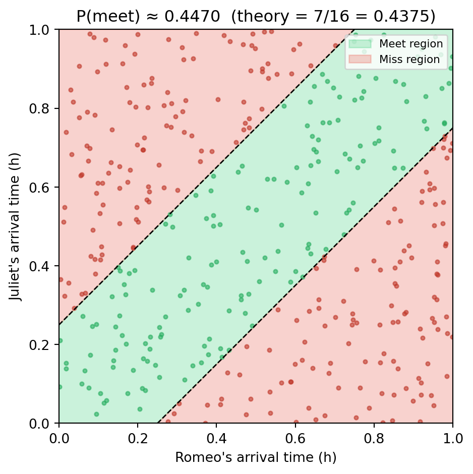
Problem (Bertsekas & Tsitsiklis, §1.2). Romeo and Juliet each arrive at a meeting place at a random time uniformly distributed in [0, 1] hour. Each will wait exactly 15 minutes (0.25 h) for the other, then leave. What is the probability they actually meet?
Step 1 — Choose the sample space.
Let x = Romeo’s arrival time and y = Juliet’s arrival time. Every pair (x, y) is equally likely, so the sample space is the unit square:
\Omega = \{(x, y) \mid 0 \le x \le 1,\ 0 \le y \le 1\}
Step 2 — Describe the event.
They meet if and only if they arrive within 15 minutes of each other:
A = \{(x, y) \in \Omega \mid |x - y| \le 0.25\}
Step 3 — Apply the geometric probability rule.
Because every point in the unit square is equally likely, probability equals area:
P(A) = \frac{\text{area of } A}{\text{area of } \Omega} = \text{area of } A
The region A is the unit square with two corner triangles removed. Each triangle has legs of length 0.75:
For the 1-D spinning wheel we argued informally: if a single value had probability c > 0, picking n > 1/c distinct values would push total probability above 1. Here are two sharper, 2-D versions of that same idea for the dart.
Suppose you throw a dart and it lands at exactly (0.5, 0.3). You might ask: what is the probability of landing at that exact point?
The answer is P(\{(0.5, 0.3)\}) = 0. Here is why this must be true — not as a definition, but as a logical consequence.
The squeezing argument. Enclose the point (0.5, 0.3) in a tiny square of side length \varepsilon. Its area is \varepsilon^2, so by the uniform law, the probability of landing inside that square is \varepsilon^2. The single point (0.5, 0.3) is a subset of that square, so:
P(\{(0.5, 0.3)\}) \le \varepsilon^2
This must hold for every\varepsilon > 0, no matter how small. The only number that is \le \varepsilon^2 for all \varepsilon > 0 is 0. So P(\{(0.5, 0.3)\}) = 0.
The additivity argument. The unit square contains uncountably many points — more than can ever be listed. If each point had even the tiniest positive probability p > 0, then summing over all points would give an infinite total probability, which contradicts P(\Omega) = 1. The only consistent assignment is p = 0 for every individual point.
What this does not mean.P = 0 does not mean the outcome is impossible. The dart does land somewhere — at some specific (x, y). It just means that in a continuous model, individual points carry no probability weight. Probability lives in regions (areas), not in isolated points.
This is the key shift from discrete to continuous thinking:
Discrete (dice)
Continuous (dart)
Outcomes are listable
Outcomes are uncountable
Each outcome can have P > 0
Each single outcome has P = 0
Probability = sum over outcomes
Probability = area of region
NoteA note on continuous events
For continuous sample spaces, a deep mathematical result shows that not every conceivable subset can be assigned a probability without breaking the axioms. This is solved by restricting events to a well-behaved collection of subsets called a \sigma-algebra. In practice, every event we can describe in this book — intervals, circles, and other geometric regions — is well-behaved. You can safely continue to think of an event as any subset of \Omega you can define. The details are in Appendix A: Foundations of Modern Probability.
3.10 Sequential Experiments and Tree Diagrams
Many real experiments unfold in stages. You don’t roll all your dice at once — you roll the first, see what happens, then roll the second. You don’t measure all your sensor outputs at once — readings come in over time. You don’t read an email and decide it’s spam in a single glance — you check the sender, then the subject line, then the body.
For these step-by-step experiments, the cleanest representation is a tree diagram. Each branch from a node represents a possible outcome at that stage; each path from root to leaf is one complete sequence of outcomes. The set of all leaves is the sample space.
Let’s draw one. We’ll use the simplest sequential experiment that’s still interesting: flipping a fair coin three times.
A few things this picture makes obvious:
Sample space is the leaves.\Omega = \{\text{HHH, HHT, HTH, HTT, THH, THT, TTH, TTT}\}, so |\Omega| = 2^3 = 8. (More generally: 2^n leaves for n tosses.)
Events are sets of leaves. “Exactly 2 heads” = \{\text{HHT, HTH, THH}\}.
Probabilities follow paths. Each branch in a fair coin tree is taken with probability 1/2, and the probability of reaching a specific leaf is the product along the path: (1/2)^3 = 1/8. Multiply along branches; add across branches.
Events are sets of leaves. “Exactly 2 heads” = \{\text{HHT, HTH, THH}\} (the medium-shaded leaves above). “At least 1 head” = all leaves except \{\text{TTT}\}.
Probabilities from equally-likely outcomes. The eight leaves are all equally likely — there is no reason to favour any one sequence over another. So each leaf gets probability \frac{1}{8} from the equally-likely formula P(A) = |A|/|\Omega|.
NoteWhy do we get 1/8 per leaf?
With 8 equally likely outcomes and a fair coin, P(\text{any single leaf}) = \frac{1}{8}.
You might notice that \frac{1}{8} = \frac{1}{2} \times \frac{1}{2} \times \frac{1}{2} — the branch probabilities multiply along the path. This is not a coincidence, but explaining why requires conditional probability, which we develop in the next chapter. Once you have that tool, we’ll come back to trees and show exactly why branch probabilities multiply down a path and why you add across paths for an event. For now, the equally-likely formula is all you need.
Let’s verify by computing some probabilities directly from the tree:
from itertools import product# Generate all leavesleaves =list(product("HT", repeat=3))print(f"Sample space size: {len(leaves)}")print(f"All leaves: {[''.join(l) for l in leaves]}")# 8 equally likely outcomes → each leaf has probability 1/8.p_leaf =1/8# Event A: exactly 2 headsevent_A = [l for l in leaves if l.count("H") ==2]print(f"\nP(exactly 2 heads) = {len(event_A)}/8 = {len(event_A)/8}")print(f" leaves: {[''.join(l) for l in event_A]}")# Event B: at least 1 headevent_B = [l for l in leaves if l.count("H") >=1]print(f"\nP(at least 1 head) = {len(event_B)}/8 = {len(event_B)/8}")# Event C: all three are the sameevent_C = [l for l in leaves if l.count("H") in (0, 3)]print(f"\nP(all same) = {len(event_C)}/8 = {len(event_C)/8}")
Trees aren’t just pictures — they’re a systematic way to enumerate sequential outcomes without missing any or double-counting. Whenever a problem can be described as “first this happens, then that, then…”, draw the tree first. The math becomes obvious.
TipWhy we’ll keep coming back to trees
Trees are the natural picture for conditional probability (the next chapter). The branches into a node from above are the conditioning; the branches out are the conditional probabilities given that you’ve arrived. Bayes’ rule is just “go up the tree and re-weight”.
3.11 The Discrete Probability Law
When the sample space is finite or countably infinite, the probability of any event is completely determined by the probabilities of individual outcomes.
ImportantDiscrete Probability Law
For a discrete sample space \Omega = \{s_1, s_2, \ldots, s_n\}, specify probabilities for each singleton event: P(\{s_i\}) \ge 0 \quad \text{for all } i, \qquad \sum_{i=1}^n P(\{s_i\}) = 1.
Then for any event A \subseteq \Omega: P(A) = \sum_{s_i \in A} P(\{s_i\}).
This is just the additivity axiom applied to the finite, pairwise disjoint singletons that make up A.
Example: a single coin toss.
\Omega = \{H, T\}. For a fair coin: P(\{H\}) = P(\{T\}) = 0.5. The axioms then force P(\emptyset) = 0 and P(\Omega) = 1. For a biased coin we might have P(\{H\}) = 0.6, P(\{T\}) = 0.4 — any assignment works as long as both values are non-negative and sum to 1.
Note▶ Three coin tosses — worked example
Toss a fair coin three times. The sample space has 2^3 = 8 equally likely outcomes: \Omega = \{HHH, HHT, HTH, HTT, THH, THT, TTH, TTT\} Each has probability 1/8.
Event
Outcomes
Probability
Exactly 2 heads
\{HHT, HTH, THH\}
3/8
At least 1 head
\Omega \setminus \{TTT\}
7/8
All same
\{HHH, TTT\}
2/8 = 1/4
from itertools import productomega_3 =list(product(['H','T'], repeat=3))p =1/len(omega_3) # 1/8 eachexactly_2H = [s for s in omega_3 if s.count('H') ==2]at_least_1H = [s for s in omega_3 if'H'in s]all_same = [s for s in omega_3 iflen(set(s)) ==1]print(f"Exactly 2 heads: {len(exactly_2H)}/8 = {len(exactly_2H)*p:.4f}")print(f"At least 1 head: {len(at_least_1H)}/8 = {len(at_least_1H)*p:.4f}")print(f"All same outcome: {len(all_same)}/8 = {len(all_same)*p:.4f}")
Exactly 2 heads:  3/8 = 0.3750
At least 1 head:  7/8 = 0.8750
All same outcome: 2/8 = 0.2500
3.12 The Discrete Uniform Law
The axioms tell us what conditions a probability law must satisfy — they do not tell us which law to use. The simplest and most common choice for a finite sample space is to treat all outcomes as equally likely.
ImportantThe Classical Probability Formula (Discrete Uniform Law)
When all outcomes in a finite sample space are equally likely, the probability of any event A is simply
P(A) \;=\; \frac{|A|}{|\Omega|} \;=\; \frac{\text{number of outcomes in } A}{\text{total number of outcomes}}.
Under the Discrete Uniform Law, probability becomes a counting problem. This is the workhorse formula behind half the probability problems you’ll ever solve — it reduces probability to combinatorics.
Example: two dice, sum = 7.
# By the equally-likely-outcomes formulaevent_sum_7 = {(d1, d2) for d1, d2 in omega if d1 + d2 ==7}p_analytical =len(event_sum_7) /36print(f"Analytical P(sum=7) = {len(event_sum_7)}/36 = {p_analytical:.6f}")print(f" = {p_analytical:.4%}")
Analytical P(sum=7) = 6/36 = 0.166667
                    = 16.6667%
Let’s verify by simulation and picture:
# Roll a million pairs of dice and count the fraction with sum = 7.n_rolls =1_000_000d1_sim = rng.integers(1, 7, size=n_rolls)d2_sim = rng.integers(1, 7, size=n_rolls)sums = d1_sim + d2_simp_empirical = (sums ==7).mean()print(f"Empirical P(sum=7) = {p_empirical:.6f} (from {n_rolls:,} rolls)")
Way 3 — Picture (where you can just see the answer).
The dice sample space animation above shows the 6×6 grid with the sum=7 diagonal highlighted — 6 blue cells out of 36. 6/36 = 1/6 \approx 0.1667. The analytical answer, the simulation, and the picture all agree.
That triangulation — formula, simulation, picture — is the working style we’ll use for the entire book. Whenever you’re unsure of an answer: simulate it. Picture it. Then prove it.
3.13 The Continuous Uniform Law
For a continuous sample space, individual outcomes have zero probability. Instead, we assign probability to regions. But why? And how do we derive the probability rule from the axioms rather than just assert it? The spinning wheel gives the cleanest answer.
3.13.1 Why single points have probability zero — the spinning wheel proof
Recall the game-show wheel: \Omega = [0,1], fair spin. Call the probability of landing on any single value c = P(\{x\}).
Step 1 — Use the axioms to bound c.
Divide [0,1] into n equal sub-intervals of length 1/n. They are pairwise disjoint and together cover \Omega, so by Additivity (A3) and Normalization (A2):
Now pick one point x_k from each sub-interval. These n singletons are disjoint, so:
P(\{x_1, \ldots, x_n\}) = nc
Since \{x_1,\ldots,x_n\} \subseteq [0,1], Monotonicity (a consequence of A3 we proved earlier) gives:
nc \le P([0,1]) = 1 \implies c \le \frac{1}{n}
Step 2 — Conclude c = 0.
This holds for every n = 1, 2, 3, \ldots The only number that satisfies c \le 1/n for all n is:
\boxed{P(\{x\}) = 0} \quad \text{for every } x \in [0,1]
Step 3 — Derive P([a,b]) = b - a.
Since single points carry no probability, probability must live in intervals. The wheel is fair — no position is special — so the probability of an interval can only depend on its length. The assignment must satisfy P([0,1]) = 1. The unique rule consistent with all three axioms and fairness is:
P(a \le X \le b) = b - a
NoteExamples
P(0.2 \le X \le 0.5) = 0.3 — a 30% arc of the wheel
P(0 \le X \le 0.25) = 0.25 — the left quarter
P(X = 0.5) = 0 — a single tick mark has zero length, zero probability
The same logic extends to two dimensions (area) and three dimensions (volume):
Sample space
Size measure
Probability rule
Interval [a, b]
Length
P(A) = \text{length}(A) / \text{length}(\Omega)
Region in \mathbb{R}^2
Area
P(A) = \text{area}(A) / \text{area}(\Omega)
Region in \mathbb{R}^3
Volume
P(A) = \text{vol}(A) / \text{vol}(\Omega)
ImportantContinuous Uniform Law
For a sample space that is a region of area 1: P(A) = \text{Area}(A)
More generally, if \Omega has area |\Omega|: P(A) = \frac{\text{Area}(A)}{\text{Area}(\Omega)}
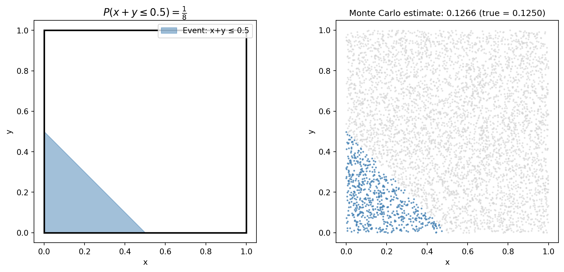
Example: Dart thrown at a unit square — \Omega = \{(x,y) \mid 0 \le x \le 1,\ 0 \le y \le 1\}, area = 1.
What is P(x + y \le 0.5)?
The event is the triangle below the line y = 0.5 - x: \text{Area} = \frac{1}{2} \times \frac{1}{2} \times \frac{1}{2} = \frac{1}{8}
What is P(\text{dart lands on exactly } (0.5, 0.3))? A single point has zero area, so P = 0. In continuous models, individual outcomes have zero probability; regions have positive probability.
import numpy as npnp.random.seed(0)n_trials =100_000outcomes_ct = []for _ inrange(n_trials): tosses =0whileTrue: tosses +=1if np.random.random() <0.5:break outcomes_ct.append(tosses)outcomes_ct = np.array(outcomes_ct)p_even = np.mean(outcomes_ct %2==0)print(f"P(even) by simulation: {p_even:.4f}")print(f"P(even) by formula: {1/3:.4f}")
P(even) by simulation: 0.3340
P(even) by formula:    0.3333
This works because the Countable Additivity Axiom lets us sum probabilities over an infinite sequence of disjoint events.
3.14.2 Why “Countable” and Not “Uncountable”?
Consider the unit square where probability = area. The square is the union of all its individual points:
\Omega = \bigcup_{(x,y) \in [0,1]^2} \{(x, y)\}
Each individual point has area (probability) = 0. If we could apply additivity to this uncountable union:
P(\Omega) = \sum_{\text{all points}} 0 = 0
But P(\Omega) = 1 by the Normalization Axiom. We get 1 = 0 — a contradiction.
The resolution: the unit square is uncountable. Its points cannot be arranged in a sequence. The Countable Additivity Axiom only applies to sequences — it does not apply here. Individual points in a continuous model simply cannot be added up to give the probability of a region; you need area (and eventually, integration).
This is exactly why the distinction between countable and uncountable sets matters for probability.
3.15 The Bonferroni Inequality
The Union Bound says: if two events are each unlikely, their union (at least one occurs) is also unlikely. The Bonferroni Inequality is the mirror image: if two events are each very likely, their intersection (both occur) is also likely.
ImportantBonferroni Inequality
For any two events A_1 and A_2: P(A_1 \cap A_2) \ge P(A_1) + P(A_2) - 1
More generally, for n events: P\!\left(\bigcap_{i=1}^n A_i\right) \ge \sum_{i=1}^n P(A_i) - (n - 1)
Proof (two events):
By De Morgan’s Law: (A_1 \cap A_2)^c = A_1^c \cup A_2^c.
By the Union Bound: P(A_1^c \cup A_2^c) \le P(A_1^c) + P(A_2^c) = (1 - P(A_1)) + (1 - P(A_2)).
Therefore: 1 - P(A_1 \cap A_2) \le 2 - P(A_1) - P(A_2), which gives the result. \blacksquare
Example: A system requires two components to both work. Component 1 works with probability 0.95, component 2 with probability 0.90. The Bonferroni Inequality gives:
P(\text{both work}) \ge 0.95 + 0.90 - 1 = 0.85
The exact answer (if independent) is 0.95 \times 0.90 = 0.855 — so the bound is tight.
Tip▶ Fun fact — Markov chains: when the past doesn’t matter
The memoryless property. Imagine a person wandering a street, taking random steps left or right. Where they go next depends only on where they are right now — not on how they got there. This is the essence of a Markov chain.
A Markov chain is a sequence of random states where: P(\text{next state} \mid \text{current state, all past states}) = P(\text{next state} \mid \text{current state})
Real-world examples:
Weather. If it’s sunny today, there’s a 70 % chance of sun tomorrow — regardless of last week’s weather.
Google PageRank. A random web surfer clicks links; the probability of visiting a page depends only on the current page, not the full browsing history.
Board games. In Monopoly, your next position depends only on where you are now and the dice roll.
Text generation (early AI). Simple autocomplete chose the next word based only on the current word.
A simple weather model. Two states: Sunny (S) and Rainy (R).
Steady state. After many steps, the chain converges to a fixed distribution — regardless of where it started. For this model: approximately 71.4 % Sunny, 28.6 % Rainy in the long run.
Code
import numpy as np# Transition matrix: rows = current state, cols = next state# State 0 = Sunny, State 1 = RainyP_markov = np.array([[0.8, 0.2], [0.5, 0.5]])# Simulate 10,000 steps starting from Sunnyrng_mc = np.random.default_rng(7)n_steps =10_000state =0# start Sunnycounts = [0, 0]for _ inrange(n_steps): state = rng_mc.choice([0, 1], p=P_markov[state]) counts[state] +=1print(f"Long-run fraction Sunny: {counts[0]/n_steps:.4f} (theory: 5/7 ≈ {5/7:.4f})")print(f"Long-run fraction Rainy: {counts[1]/n_steps:.4f} (theory: 2/7 ≈ {2/7:.4f})")
Markov chains appear in ML (Hidden Markov Models for speech recognition), finance (credit rating transitions), biology (DNA sequence modelling), and physics (statistical mechanics). Named after Russian mathematician Andrey Markov (1856–1922), who first studied them while analysing the pattern of vowels and consonants in Russian literature.
3.16 Three things you should take away
Probability has two interpretations and one math. Frequentist probability is a long-run frequency; subjective probability is a degree of belief. They argue about Stage 1 (modelling). They agree on Stage 2 (the math).
Every probability calculation rests on three things — sample space, events, axioms. Specify the first two carefully; the third is non-negotiable. Most “paradoxes” come from being sloppy about \Omega.
Simulation is your safety net. When in doubt, write a population, simulate it, count what’s in each bucket. The closed-form answers in the rest of this book are descriptions of those counts.
3.17 Exercises
1. Build a sample space. Define \Omega for the experiment “draw one card from a standard 52-card deck”. Then describe the following events as subsets: (a) the card is a heart; (b) the card is a face card (J, Q, K); (c) the card is a red ace. Compute P(\cdot) for each, assuming all cards are equally likely.
2. Frequentist limit. Modify the coin-convergence simulation above to use a biased coin with p = 0.3. Plot the running frequency. How many flips do you need before the frequency is within 0.01 of the true value? Run it 5 times — does the answer vary?
3. Check an axiom. Pick any two events from the dice example (e.g. E = “sum is even” and F = “first die is odd”). Verify inclusion–exclusion: compute P(E), P(F), P(E \cap F), and P(E \cup F) separately, and check that P(E \cup F) = P(E) + P(F) - P(E \cap F).
4. Sample space design. A bag contains 3 red balls and 2 blue balls. You draw two balls without replacement. (a) Define a sample space that tracks which specific balls are drawn and in what order. (b) Define a simpler sample space that only tracks the colours (not which specific ball). (c) Which sample space would you use to answer: “What is the probability both balls are red?” (d) Compute that probability.
5. Countable additivity. A biased coin has P(\text{heads}) = p on each toss. You toss until the first heads. (a) Write down P(n) — the probability the first heads appears on toss n. (b) Verify that \sum_{n=1}^{\infty} P(n) = 1 (use the geometric series formula). (c) Find the probability the experiment ends on an odd toss.
6. Continuous probability. A point (x, y) is chosen uniformly at random from the unit square [0,1]^2. (a) Find P(x^2 + y^2 \le 1) — the probability the point falls inside the unit circle. (Hint: what fraction of the square does the quarter-circle occupy?) (b) Write a Monte Carlo simulation to estimate this probability. (c) What famous constant does your answer approximate?
7. Bonferroni in engineering. A message is sent through 3 independent communication channels. Each channel delivers the message correctly with probability 0.8. The message is successfully received if all three channels deliver it correctly. (a) Use the Bonferroni Inequality to find a lower bound on P(\text{success}). (b) Compute the exact probability (using independence). (c) How tight is the bound?
3.18 Math Refresher
This section reviews the mathematical background needed throughout the probability chapters. It is placed here deliberately — after you have seen probability in action, the reason for each tool is clearer. Return to any subsection when you need it.
3.18.1 Set Theory
Definitions and notation
A set is a collection of distinct elements. We write x \in S if x is an element of S, and x \notin S if it is not.
Sets can be specified by listing: S = \{1, 2, 3\}, or by property: S = \{x \in \mathbb{R} \mid \cos(x) > 0\}.
Special sets:
Universal set\Omega: all objects under consideration (the sample space in probability).
Empty set\emptyset: the set containing no elements.
ComplementS^c: everything in \Omega not in S.
Subsets and equality
S \subseteq T means every element of S is also in T. Two sets are equal (S = T) iff S \subseteq T and T \subseteq S.
Operations
Operation
Symbol
Definition
Union
S \cup T
\{x \mid x \in S \text{ or } x \in T\}
Intersection
S \cap T
\{x \mid x \in S \text{ and } x \in T\}
Complement
S^c
\{x \in \Omega \mid x \notin S\}
Difference
S \setminus T
S \cap T^c
For infinite collections: \bigcup_{n=1}^\infty S_n = \{x \mid x \in S_n \text{ for some } n\} and \bigcap_{n=1}^\infty S_n = \{x \mid x \in S_n \text{ for all } n\}.
Algebraic properties
Commutativity: S \cup T = T \cup S, S \cap T = T \cap S
Associativity: (S \cup T) \cup U = S \cup (T \cup U)
Distributivity: S \cap (T \cup U) = (S \cap T) \cup (S \cap U)
Identity: S \cup \emptyset = S, S \cap \Omega = S
Domination: S \cup \Omega = \Omega, S \cap \emptyset = \emptyset
Double complement: (S^c)^c = S
3.18.2 De Morgan’s Laws
These laws convert between unions and intersections via complements. They are used constantly in probability when it is easier to compute the complement of an event.
\boxed{(S \cap T)^c = S^c \cup T^c}
\boxed{(S \cup T)^c = S^c \cap T^c}
Intuition for the first law: “Not (both S and T)” is the same as “not S, or not T.”
Key use in probability: To find P(A \cap B), sometimes it is easier to find P((A \cap B)^c) = P(A^c \cup B^c) and subtract from 1. De Morgan’s makes this switch legal.
3.18.3 Sequences and Convergence
A sequence is a function from the positive integers to some set: a_1, a_2, a_3, \ldots
Convergence: A sequence \{a_i\} converges to a if the values get arbitrarily close to a and stay there:
\lim_{i \to \infty} a_i = a \quad \Longleftrightarrow \quad \forall \epsilon > 0,\ \exists i_0 : |a_i - a| < \epsilon \text{ for all } i \ge i_0
Key properties (if a_i \to a and b_i \to b):
a_i + b_i \to a + b
a_i \cdot b_i \to a \cdot b
g(a_i) \to g(a) for any continuous function g
Monotone convergence: A non-decreasing, bounded sequence always converges. This is why the partial sums of a non-negative series always have a well-defined limit (possibly \infty).
Squeeze theorem: If x_i \le a_i \le y_i and x_i \to a and y_i \to a, then a_i \to a.
3.18.4 Infinite Series
An infinite series is the limit of its partial sums:
Non-negative series: If a_i \ge 0, the partial sums are non-decreasing, so the limit always exists (it may be \infty). For probability, we need it to be finite and equal to 1.
Absolute convergence: A series \sum a_i is absolutely convergent if \sum |a_i| < \infty. Absolute convergence guarantees:
The series converges to a finite value.
The value is the same regardless of the order in which terms are added.
In probability models, absolute convergence is the standard assumption that makes all manipulations safe.
Derivation (algebraic trick): Let S = 1 + \alpha + \alpha^2 + \cdots. Then \alpha S = \alpha + \alpha^2 + \cdots, so S - \alpha S = 1, giving S = \frac{1}{1-\alpha}.
Useful variation (starting at i = k): \sum_{i=k}^\infty \alpha^i = \frac{\alpha^k}{1 - \alpha}
This series appears constantly in probability — any time you count “the number of trials until the first success.”
Example: For the coin-toss problem, P(\text{even}) = \sum_{k=1}^\infty (1/2)^{2k} = \sum_{k=1}^\infty (1/4)^k = \frac{1/4}{1 - 1/4} = \frac{1}{3}.
3.18.6 Double Series
When summing over two indices i and j, you can sum row by row or column by column. If the series is absolutely convergent, the order does not matter:
This identity is used frequently when computing expectations and joint probabilities of discrete random variables.
3.18.7 Countable and Uncountable Sets
A set is countable if its elements can be put in a one-to-one correspondence with the positive integers — equivalently, if they can be arranged in a sequence s_1, s_2, s_3, \ldots
Examples of countable sets:
The positive integers \{1, 2, 3, \ldots\} — trivially.
The integers \mathbb{Z} — arrange as 0, 1, -1, 2, -2, 3, -3, \ldots
Pairs of positive integers — zigzag diagonally through the grid.
The rational numbers \mathbb{Q} — list by denominator, skip duplicates.
A set is uncountable if it is infinite but cannot be arranged in a sequence.
Examples of uncountable sets:
Any interval [a, b] with a < b on the real line.
The real numbers \mathbb{R}.
The plane \mathbb{R}^2, space \mathbb{R}^3, etc.
Why this matters for probability:
Sample space type
How to assign probability
Model type
Finite
Assign p_i \ge 0 to each outcome, sum = 1
Discrete
Countably infinite
Same, using an infinite sum
Discrete
Uncountably infinite
Assign probability to regions (area/length/volume)
Continuous
The Countable Additivity Axiom works for sequences. It fails for uncountable collections — which is why continuous models require integration, not summation.
3.18.8 Cantor’s Diagonal Argument
Claim: The unit interval (0, 1) is uncountable.
Proof by contradiction: Suppose all real numbers in (0,1) whose decimal expansions contain only the digits 3 and 4 could be listed in a sequence x_1, x_2, x_3, \ldots
Construct a new number y by looking at the diagonal (bolded digits) and flipping each: if the diagonal digit is 3, write 4; if it is 4, write 3.
From the example above: y = 0.4344\ldots
Now: y differs from x_1 in the 1st digit, from x_2 in the 2nd digit, from x_n in the n-th digit — so y \ne x_n for every n. Yet y consists only of 3s and 4s, so it belongs in our set. Contradiction — the list was supposed to contain everything, but y is missing.
Therefore no such list can exist. The set is uncountable. \blacksquare
The same argument applies to the full real line, establishing that \mathbb{R} is uncountably infinite — a fundamentally larger kind of infinity than the integers or rationals.
_-_Gu%C3%A9rin.jpg)