9  Central Limit Theorem

9.1 An applied scenario — smoothing the vibration stream

Back to the running motor. The raw accelerometer stream is jagged — every sample is a noisy snapshot. To get a stable reading you do the obvious thing: take a moving average over the last n samples.

Try n = 10. The output is calmer than the raw stream but still bumpy. Try n = 100. Calmer still. Try n = 1000 and the smoothed signal is almost glassy.

Two things happen as n grows:

1. The spread of the smoothed signal shrinks. Doubling n shrinks the spread by \sqrt{2}.
2. The shape of the smoothed signal’s distribution converges to a clean bell curve — even if the raw samples have a weird, skewed, or bimodal distribution.

The first observation is intuitive. The second is much deeper, and it’s the most useful theorem in all of probability.

---

9.2 The theorem

The Central Limit Theorem (CLT) says: if you sum or average many independent random variables, the result is approximately Normal — regardless of what distribution the individual variables came from.

Let X_1, X_2, \ldots, X_n be independent with mean \mu and variance \sigma^2. Then as n \to \infty, the sample mean \bar{X} = \frac{1}{n}\sum X_i converges to:

\bar{X} \;\sim\; \mathcal{N}\!\left(\mu, \frac{\sigma^2}{n}\right)

Or equivalently, the sum S_n = \sum X_i converges to:

S_n \;\sim\; \mathcal{N}(n\mu, \, n\sigma^2)

The individual X_i can be from any distribution — uniform, exponential, Poisson, Bernoulli, even something bizarre and bimodal. As long as you sum enough of them, the result is Gaussian.

---

9.3 Back to the smoothed vibration

For the moving-average filter on the accelerometer stream:

• \sigma^2 — variance of one raw sample
• n — window length
• Smoothed sample variance: \sigma^2 / n
• Smoothed sample standard deviation: \sigma / \sqrt n

That’s the 1/\sqrt n noise reduction law, and it falls out of the CLT for free. Want half the noise? Quadruple the window. Want a tenth of the noise? Multiply the window by 100.

It’s also why a smoothed signal looks Gaussian-distributed even when the raw stream is wildly non-Gaussian (impulsive transients, clipped values, mixed regimes). Averaging always pulls you toward the bell.

---

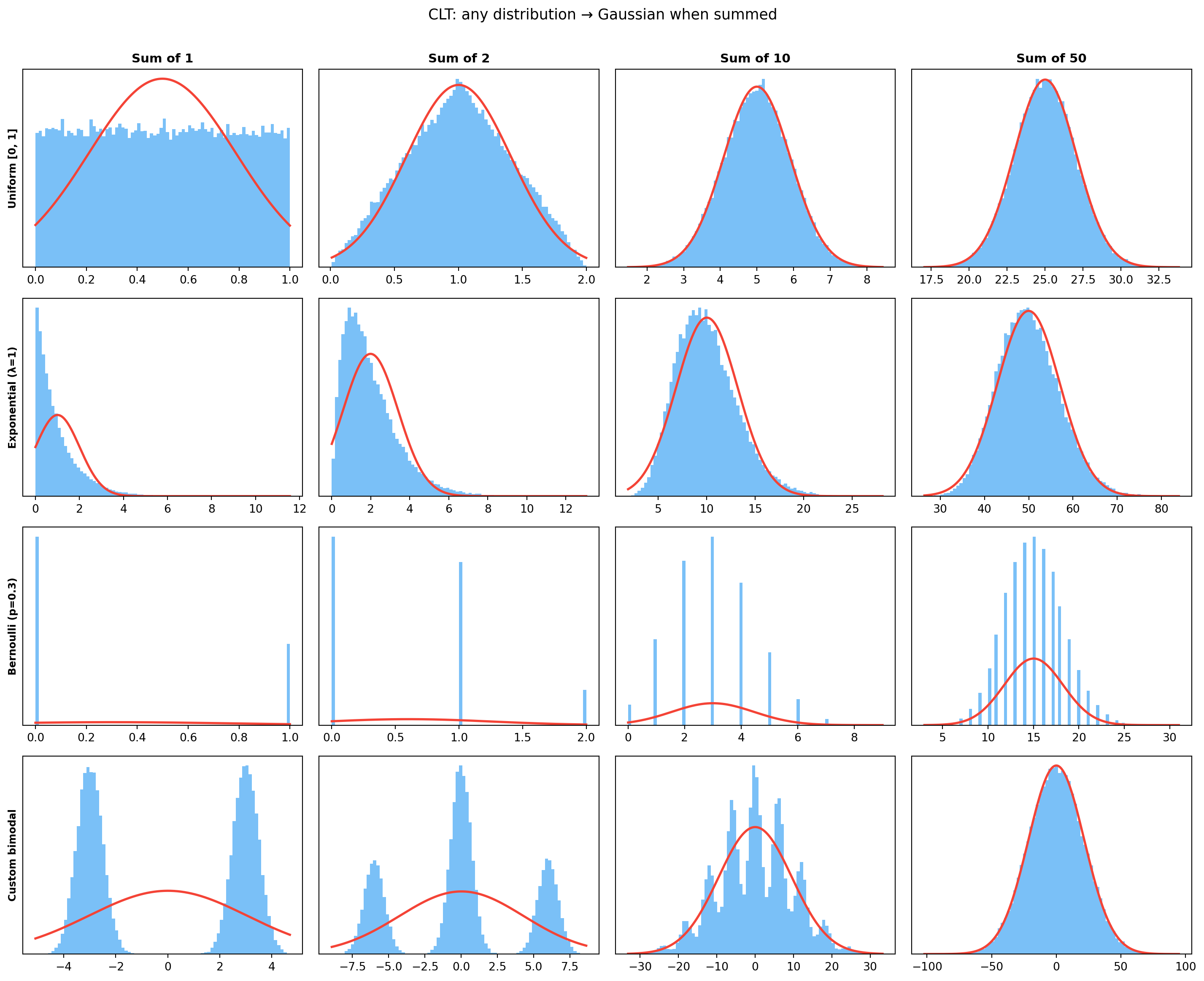
9.4 CLT in action — sums of non-Gaussian variables

import numpy as np
import matplotlib.pyplot as plt
from scipy.stats import norm, kstest

np.random.seed(42)
n_samples = 50_000

distributions = {
    "Uniform [0, 1]":   lambda s: np.random.uniform(0, 1, s),
    "Exponential (λ=1)": lambda s: np.random.exponential(1, s),
    "Bernoulli (p=0.3)": lambda s: np.random.binomial(1, 0.3, s),
    "Custom bimodal":   lambda s: np.where(np.random.random(s) < 0.5,
                                           np.random.normal(-3, 0.5, s),
                                           np.random.normal(3, 0.5, s)),
}

fig, axes = plt.subplots(len(distributions), 4, figsize=(15, 12))
n_sums = [1, 2, 10, 50]

for row, (name, sampler) in enumerate(distributions.items()):
    for col, n in enumerate(n_sums):
        total = np.zeros(n_samples)
        for _ in range(n):
            total += sampler(n_samples)

        ax = axes[row, col]
        ax.hist(total, bins=80, density=True, color="#2196F3", alpha=0.6)
        xr = np.linspace(total.min(), total.max(), 300)
        ax.plot(xr, norm.pdf(xr, total.mean(), total.std()),
                color="#F44336", linewidth=2)
        if row == 0:
            ax.set_title(f"Sum of {n}", fontsize=11, fontweight="bold")
        if col == 0:
            ax.set_ylabel(name, fontsize=9, fontweight="bold")
        ax.set_yticks([])

plt.suptitle("CLT: any distribution → Gaussian when summed",
             fontsize=13, y=1.005)
plt.tight_layout()
plt.show()

Each row starts non-Gaussian. By column 4 (sum of 50), every distribution looks like a clean bell — the CLT, regardless of where you started.

---

9.5 CLT explains Poisson → Normal

The Poisson(\lambda) random variable can be thought of as the sum of \lambda independent Poisson(1) variables. By the CLT, this sum converges to \mathcal{N}(\lambda, \lambda) as \lambda \to \infty. The Poisson-to-Normal convergence from the previous chapter is just one instance of the same theorem.

---

9.6 A sensor reading is already a sum

A single reading from almost any sensor is itself a sum of many independent contributions:

\text{reading} \;=\; \underbrace{\text{primary signal}}_{\text{the thing you want}} + \underbrace{\sum_{i} \eta_i}_{\text{thermal / electronic noise}} + \underbrace{\sum_{j} d_j}_{\text{interference / drift}} + \underbrace{q}_{\text{quantization}}

By the CLT the total error is approximately Gaussian even though the individual sources have completely different distributions. This is the deeper reason every classical signal-processing tool — Wiener, Kalman, Gaussian denoising, least-squares — assumes Gaussian noise.

---

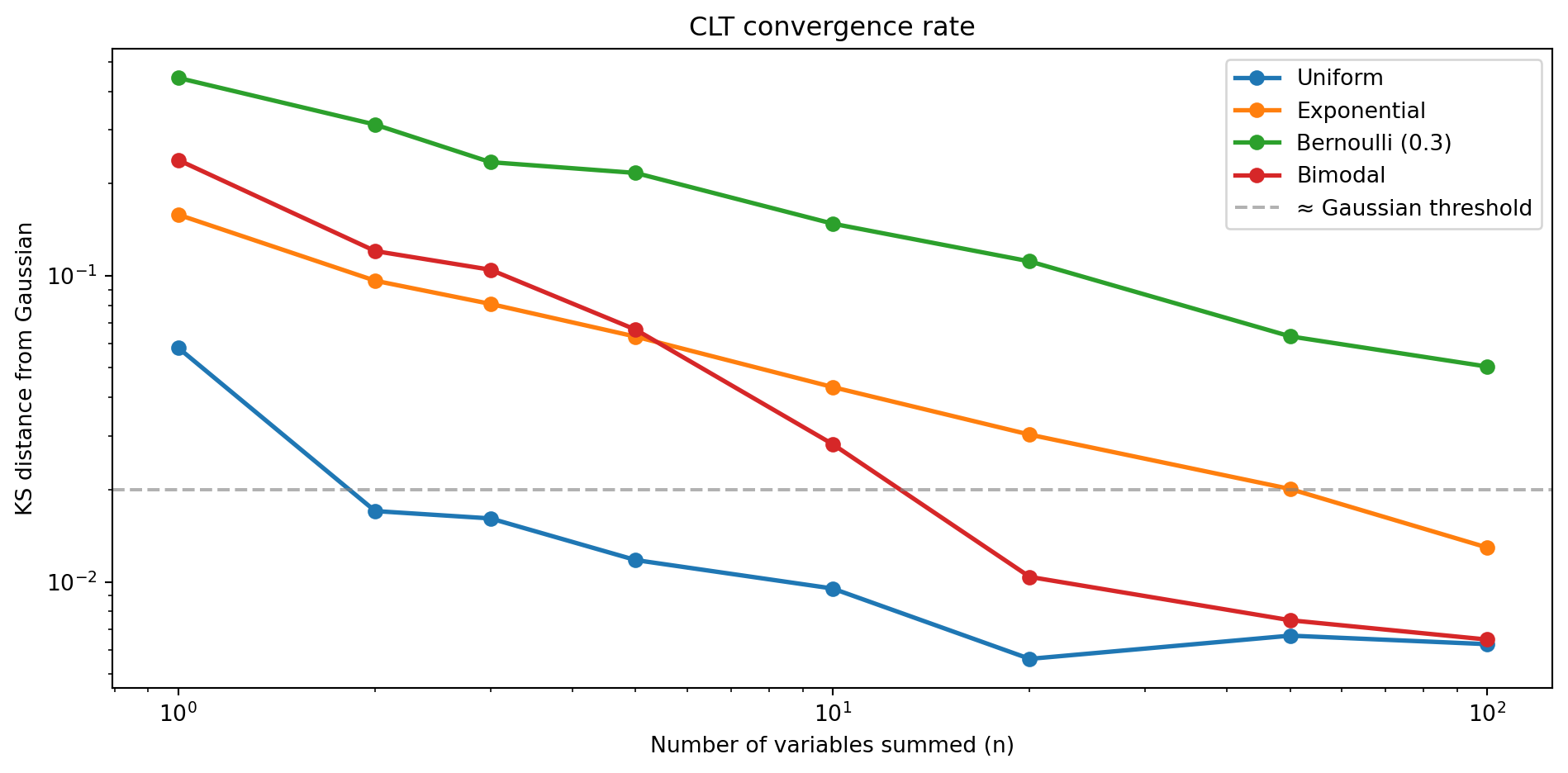
9.7 Convergence rate

Convergence to Normal is fast for some distributions and slow for others. The rate depends on the skewness of the original distribution.

n_values = [1, 2, 3, 5, 10, 20, 50, 100]
dist_fns = {
    "Uniform":         lambda s: np.random.uniform(0, 1, s),
    "Exponential":     lambda s: np.random.exponential(1, s),
    "Bernoulli (0.3)": lambda s: np.random.binomial(1, 0.3, s),
    "Bimodal":         lambda s: np.where(np.random.random(s) < 0.5,
                                          np.random.normal(-3, 0.5, s),
                                          np.random.normal(3, 0.5, s)),
}

fig, ax = plt.subplots(figsize=(10, 5))

for name, sampler in dist_fns.items():
    ks = []
    for n in n_values:
        total = np.zeros(10_000)
        for _ in range(n):
            total += sampler(10_000)
        z = (total - total.mean()) / total.std()
        ks_stat, _ = kstest(z, "norm")
        ks.append(ks_stat)
    ax.plot(n_values, ks, "o-", linewidth=2, markersize=6, label=name)

ax.axhline(0.02, color="grey", linestyle="--", alpha=0.6,
           label="≈ Gaussian threshold")
ax.set_xlabel("Number of variables summed (n)")
ax.set_ylabel("KS distance from Gaussian")
ax.set_title("CLT convergence rate")
ax.set_xscale("log")
ax.set_yscale("log")
ax.legend()
plt.tight_layout()
plt.show()

Symmetric distributions (Uniform) converge fastest; skewed (Exponential) slower; bimodal slowest. KS distance below ≈ 0.02 means effectively Gaussian for downstream tools.

The convergence rate is approximately O(1/\sqrt n). In practical terms, this tells you how long a moving-average window needs to be before the smoothed output is genuinely Gaussian, or how many frames to average before a Gaussian-based background-subtraction model is valid.

---

9.8 Exercises

1. For X \sim \text{Uniform}[0, 1], simulate the sample mean of n = 5, 30, 100 samples 10 000 times each. Plot the three sampling distributions on the same axes.
2. Verify the 1/\sqrt n rule: plot the std of the sample mean vs n on a log-log scale; the slope should be -1/2.
3. Run a KS test on standardised sums of an exponential distribution. At what n does the KS statistic drop below 0.02?
4. Sums of Cauchy random variables do not become Gaussian. Why? (Hint: think about the assumption “finite variance”.)

---

9.9 Glossary

CLT — sample mean of many i.i.d. variables is approximately Normal.

i.i.d. — independent and identically distributed.

1/\sqrt n rule — std of sample mean shrinks as \sigma / \sqrt n.

KS distance — Kolmogorov–Smirnov statistic; max gap between empirical and theoretical CDF.

convergence rate — how fast the limit is approached as n grows.