6  Binomial — Counting Successes

6.1 An applied scenario — one second of vibration samples

Back to the motor from the last chapter. The accelerometer streams 1 000 samples per second, and your threshold rule fires a 1 whenever a sample exceeds +2\,\mathrm{g}. On a healthy machine, calibration gave you p = 0.005 (1 in 200 samples is a transient).

You decide to summarise the stream one second at a time: count how many 1s show up in each 1 000-sample window. That count is the alarm metric the operator sees.

A few obvious questions:

• What count should you expect on a healthy machine?
• How much can the count drift from one second to the next without anything actually being wrong?
• If you see a count of 20 in one window, is that worrying — or just normal variation?

Each window is n = 1000 independent Bernoulli trials with p = 0.005. The thing you’re counting — successes out of n trials — has a name.

---

6.2 Intuition

If a Bernoulli trial is one coin flip, the Binomial distribution answers: “If I run n independent trials, each with success probability p, how many successes will I get?”

• Vibration window: in 1 000 samples, each with probability p = 0.005 of crossing the threshold, how many crossings k?
• Manufacturing batch: 200 units, each defective with probability p = 0.02, how many defects k?
• Photon counting: n photons strike a sensor and each has probability p = \text{QE} of being detected, how many electrons k?

In every case the structure is identical: n independent Bernoulli trials with the same p, count the successes.

---

6.3 The math

P(k \mid n, p) \;=\; \binom{n}{k} p^k (1-p)^{n-k}

where \binom{n}{k} = \frac{n!}{k!(n-k)!} is the number of ways to choose which k out of n trials succeed.

Mean: E[k] = np

Variance: \operatorname{Var}(k) = np(1-p)

Breaking the formula down:

• \binom{n}{k} — how many ways exactly k trials can succeed out of n total
• p^k — probability that those k trials all succeed
• (1-p)^{n-k} — probability that the remaining n-k trials all fail
• multiply: total probability of exactly k successes

Note▶ Show the math — E[k] = np from the Bernoulli sum

A Binomial random variable is just the sum of n independent Bernoulli(p) trials:

K \;=\; X_1 + X_2 + \cdots + X_n, \quad X_i \sim \text{Bernoulli}(p)

Linearity of expectation gives E[K] = nE[X_1] = np directly. Independence then gives \operatorname{Var}(K) = n\operatorname{Var}(X_1) = np(1-p).

---

6.4 Build the PMF term by term

import numpy as np
import matplotlib.pyplot as plt
from scipy.stats import binom
from scipy.special import comb

np.random.seed(42)

n = 10
p = 0.7   # photon QE — the cleanest example we have

print(f"n = {n} photons, p = {p} (QE)")
print()
print(f"{'k':>4}  {'C(n,k)':>8}  {'p^k':>10}  {'(1-p)^(n-k)':>14}  {'P(k)':>10}")
print("-" * 56)
for k in range(n + 1):
    ways      = comb(n, k, exact=True)
    p_succ    = p ** k
    p_fail    = (1 - p) ** (n - k)
    prob      = ways * p_succ * p_fail
    print(f"{k:>4}  {ways:>8}  {p_succ:>10.6f}  {p_fail:>14.6f}  {prob:>10.6f}")

print()
print(f"Expected: np      = {n * p}")
print(f"Variance: np(1-p) = {n * p * (1 - p):.4f}")
print(f"Std dev : √var    = {np.sqrt(n * p * (1 - p)):.4f}")

n = 10 photons, p = 0.7 (QE)

   k    C(n,k)         p^k     (1-p)^(n-k)        P(k)
--------------------------------------------------------
   0         1    1.000000        0.000006    0.000006
   1        10    0.700000        0.000020    0.000138
   2        45    0.490000        0.000066    0.001447
   3       120    0.343000        0.000219    0.009002
   4       210    0.240100        0.000729    0.036757
   5       252    0.168070        0.002430    0.102919
   6       210    0.117649        0.008100    0.200121
   7       120    0.082354        0.027000    0.266828
   8        45    0.057648        0.090000    0.233474
   9        10    0.040354        0.300000    0.121061
  10         1    0.028248        1.000000    0.028248

Expected: np      = 7.0
Variance: np(1-p) = 2.1000
Std dev : √var    = 1.4491

scipy.stats.binom.pmf does exactly these steps internally. Seeing it once makes the formula concrete.

---

6.5 Back to the vibration sensor

For the motor:

n = 1000, \quad p = 0.005 \;\Rightarrow\; E[k] = 5, \quad \operatorname{Var}(k) \approx 4.975, \quad \sigma \approx 2.23

So on a healthy machine you should see about 5 crossings per second with a typical fluctuation of \pm 2. A count of 7 is unremarkable. A count of 20 is roughly 7\sigma above the mean — not normal variation, that’s a state change worth investigating.

---

6.6 How shape changes with n and p

fig, axes = plt.subplots(2, 3, figsize=(15, 8))

p_fixed = 0.7
for ax, n_var in zip(axes[0], [5, 20, 100]):
    k = np.arange(0, n_var + 1)
    ax.bar(k, binom.pmf(k, n_var, p_fixed), color="#2196F3", alpha=0.85)
    mu = n_var * p_fixed
    ax.axvline(mu, color="#F44336", linestyle="--", linewidth=2)
    ax.set_title(f"n = {n_var}, p = {p_fixed}")
    ax.set_xlabel("k")
    ax.set_ylabel("P(k)")

n_fixed = 30
for ax, p_var in zip(axes[1], [0.1, 0.5, 0.9]):
    k = np.arange(0, n_fixed + 1)
    ax.bar(k, binom.pmf(k, n_fixed, p_var), color="#4CAF50", alpha=0.85)
    mu = n_fixed * p_var
    ax.axvline(mu, color="#F44336", linestyle="--", linewidth=2)
    ax.set_title(f"n = {n_fixed}, p = {p_var}")
    ax.set_xlabel("k")
    ax.set_ylabel("P(k)")

plt.tight_layout()
plt.show()

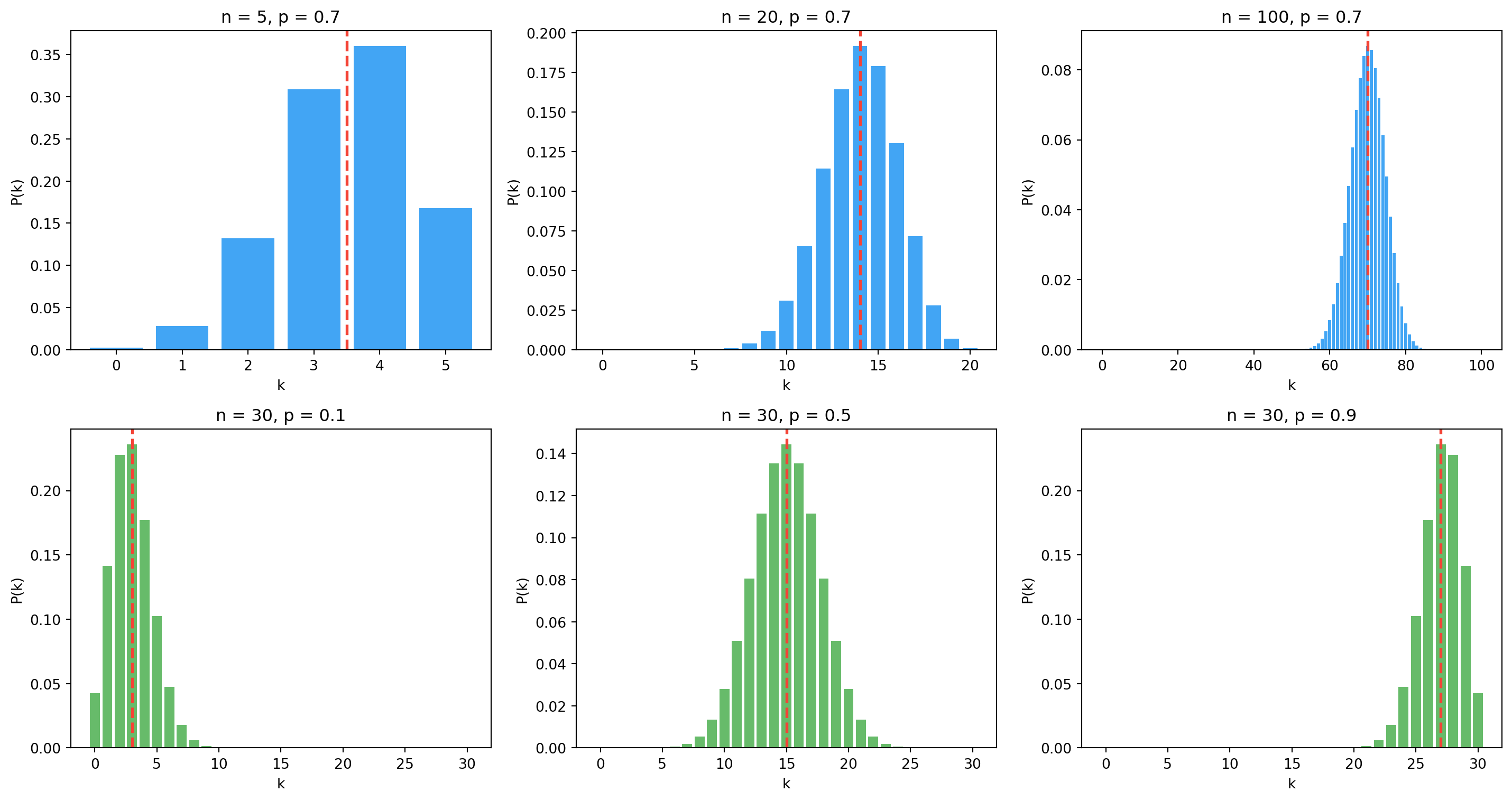
Top row: fix p = 0.7, vary n. Distribution widens and becomes more bell-shaped (CLT preview). Bottom row: fix n = 30, vary p. Peak shifts; symmetric at p = 0.5.

For the motor case, p = 0.005 and n = 1000 — the distribution is heavily skewed and concentrated near small counts. That regime — many trials, each rare — is exactly where the Binomial morphs into the Poisson distribution (next chapter).

---

6.7 Simulation — repeated windows

Simulating many 1-second windows is the empirical version of the formula. Each simulated window is one independent set of n Bernoulli trials.

np.random.seed(42)
n_phot = 100
qe = 0.7
n_exp = 10_000

electron_counts = np.random.binomial(n_phot, qe, size=n_exp)

print(f"{n_exp:,} exposures simulated")
print(f"  Mean : {electron_counts.mean():.2f}  (theory {n_phot * qe})")
print(f"  Std  : {electron_counts.std():.2f}   (theory "
      f"{np.sqrt(n_phot * qe * (1 - qe)):.2f})")

10,000 exposures simulated
  Mean : 69.93  (theory 70.0)
  Std  : 4.56   (theory 4.58)

k_values = np.arange(electron_counts.min(), electron_counts.max() + 1)
theoretical = binom.pmf(k_values, n_phot, qe)

fig, axes = plt.subplots(1, 2, figsize=(13, 4))

axes[0].hist(electron_counts, bins=k_values - 0.5, density=True,
             color="#2196F3", alpha=0.5, label="Simulated")
axes[0].plot(k_values, theoretical, "o-", color="#F44336",
             markersize=4, linewidth=2, label="Theory")
axes[0].set_xlabel("Electrons per exposure")
axes[0].set_ylabel("Probability")
axes[0].set_title(f"Binomial({n_phot}, {qe})")
axes[0].legend()

axes[1].hist(electron_counts, bins=k_values - 0.5, density=True,
             cumulative=True, color="#2196F3", alpha=0.5, label="Simulated CDF")
axes[1].plot(k_values, binom.cdf(k_values, n_phot, qe),
             "-", color="#F44336", linewidth=2, label="Theoretical CDF")
axes[1].set_xlabel("Electrons per exposure")
axes[1].set_ylabel("P(X ≤ k)")
axes[1].set_title("CDF")
axes[1].legend()

plt.tight_layout()
plt.show()

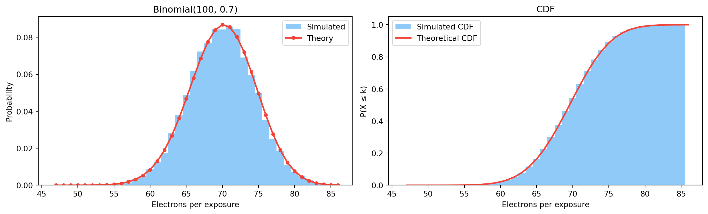
Simulation histogram (bars) hugs the theoretical Binomial PMF (line); residual differences shrink as the number of simulated windows grows (CLT effect).

TipWhy simulate when we have the formula?

Simulation validates the theory and builds intuition. If simulation and formula disagree, one of them is wrong — a debugging technique that survives all the way into deep learning, where closed-form answers stop existing and Monte Carlo is the only tool.

---

6.8 Where else binomial counts appear

Domain	n	p	Count k
Vibration monitoring	Samples per window	P(threshold crossing)	Crossings per window
Quality control	Units per batch	P(defective)	Defects per batch
A/B testing	Visitors in a bucket	P(conversion)	Conversions per bucket
Image thresholding	Pixels in a patch	P(intensity > T)	Bright pixels per patch
Photon counting	Incident photons	Quantum efficiency	Detected electrons

The formula doesn’t care what the trial is — only that the trials are independent and share the same p. When p varies across trials or trials aren’t independent, you need a different model.

---

6.9 Exercises

1. Manually compute P(k = 3) for n = 10, p = 0.4. Confirm against scipy.stats.binom.pmf.
2. For n = 1000 and p = 0.005, simulate 10\,000 windows. What fraction of windows produce a count \geq 20?
3. Plot Binomial PMFs for p = 0.5 at n = 5, 20, 100, 500. Watch the convergence to bell shape.
4. Show by simulation that mean and variance match np and np(1-p) to within Monte Carlo error.

---

6.10 Glossary

Binomial distribution — count of successes in n independent Bernoulli trials with constant p.

n — number of trials.

p — success probability per trial.

k — number of successes (random).

PMF — probability mass function P(k).

CDF — cumulative distribution function P(X \leq k).