18  Cumulative Distribution Functions

18.1 The limits of PMFs

PMFs work well for discrete data with few unique values (like pregnancy length in weeks). But for continuous data — birth weight in pounds — there can be hundreds of distinct values, and plotting every one gives a noisy, unreadable picture.

We need a representation that:

1. Works for any data (discrete or continuous)
2. Makes it easy to compare distributions visually
3. Supports questions like “what percentile is 8 lbs?”

The Cumulative Distribution Function (CDF) does all three.

---

18.2 What is a CDF?

The CDF answers one question: what fraction of the data is at or below a given value?

F(x) \;=\; P(X \leq x)

For empirical data this is just:

F(x) \;=\; \frac{\text{number of values} \leq x}{n}

The CDF is always non-decreasing, between 0 and 1, starts at 0, and ends at 1.

---

18.3 Building a CDF from scratch

import sys, os
import numpy as np
import matplotlib.pyplot as plt

sys.path.insert(0, os.path.dirname(os.path.abspath("__file__")) or ".")
from _nsfg import load_groups, COLORS

live, first, other = load_groups()


class Cdf:
    """Empirical CDF: F(x) = fraction of values <= x."""

    def __init__(self, values):
        clean = np.array(sorted(v for v in values if not np.isnan(float(v))))
        n = len(clean)
        self.xs = clean
        self.ps = np.arange(1, n + 1) / n   # rank / n

    def prob(self, x: float) -> float:
        idx = np.searchsorted(self.xs, x, side="right")
        return idx / len(self.xs)

    def value(self, p: float) -> float:
        if p <= 0:
            return self.xs[0]
        if p >= 1:
            return self.xs[-1]
        idx = int(p * len(self.xs))
        return self.xs[idx]

    def median(self) -> float:
        return self.value(0.5)

    def iqr(self) -> float:
        return self.value(0.75) - self.value(0.25)

    def percentile_rank(self, x: float) -> float:
        return self.prob(x) * 100

    def sample(self, n: int) -> np.ndarray:
        u = np.random.uniform(0, 1, size=n)
        return np.array([self.value(ui) for ui in u])


wgt_cdf_all   = Cdf(live["totalwgt_lb"].dropna().values)
wgt_cdf_first = Cdf(first["totalwgt_lb"].dropna().values)
wgt_cdf_other = Cdf(other["totalwgt_lb"].dropna().values)

prg_cdf_first = Cdf(first["prglngth"].dropna().values)
prg_cdf_other = Cdf(other["prglngth"].dropna().values)
print(f"All babies: n = {len(wgt_cdf_all.xs):,}")

All babies: n = 9,087

Every value gets a rank. The CDF at value x is rank divided by n.

---

18.4 Percentiles

A percentile is the inverse CDF: given a probability p, find the value x such that F(x) = p.

• 50th percentile = median — half the data is below this value
• 25th percentile = first quartile (Q1)
• 75th percentile = third quartile (Q3)
• IQR = Q3 − Q1 = the middle 50% of the data

print("── Birth Weight: Percentile Summary ─────────────────────")
for label, cdf in [("All babies", wgt_cdf_all),
                   ("First babies", wgt_cdf_first),
                   ("Other babies", wgt_cdf_other)]:
    print(f"\n  {label}:")
    print(f"    25th percentile : {cdf.value(0.25):.2f} lbs")
    print(f"    Median  (50th)  : {cdf.median():.2f} lbs")
    print(f"    75th percentile : {cdf.value(0.75):.2f} lbs")
    print(f"    IQR             : {cdf.iqr():.2f} lbs")

── Birth Weight: Percentile Summary ─────────────────────

  All babies:
    25th percentile : 6.50 lbs
    Median  (50th)  : 7.38 lbs
    75th percentile : 8.12 lbs
    IQR             : 1.62 lbs

  First babies:
    25th percentile : 6.44 lbs
    Median  (50th)  : 7.31 lbs
    75th percentile : 8.00 lbs
    IQR             : 1.56 lbs

  Other babies:
    25th percentile : 6.50 lbs
    Median  (50th)  : 7.38 lbs
    75th percentile : 8.25 lbs
    IQR             : 1.75 lbs

So the typical newborn weighs between roughly 6.4 and 8.1 lbs.

---

18.5 Comparing CDFs

The real power of the CDF: two CDFs on the same plot tell the whole story. For pregnancy length, plot first vs other on one axis. If the curves are nearly identical, the difference between groups is tiny.

print("── Where Does a Specific Weight Rank? ───────────────────")
for w in [6.0, 7.0, 7.5, 8.0, 9.0, 10.0]:
    print(f"  A baby weighing {w:.1f} lbs is at the "
          f"{wgt_cdf_all.percentile_rank(w):.1f}th percentile")

── Where Does a Specific Weight Rank? ───────────────────
  A baby weighing 6.0 lbs is at the 14.4th percentile
  A baby weighing 7.0 lbs is at the 40.0th percentile
  A baby weighing 7.5 lbs is at the 57.5th percentile
  A baby weighing 8.0 lbs is at the 72.9th percentile
  A baby weighing 9.0 lbs is at the 92.0th percentile
  A baby weighing 10.0 lbs is at the 97.9th percentile

---

18.6 Generating data from a CDF

A useful trick: if U is a uniform random number between 0 and 1, then F^{-1}(U) has the same distribution as the original data. This lets us simulate new data that matches an observed distribution — the foundation of bootstrap (Chapter 8).

np.random.seed(42)
synthetic = wgt_cdf_all.sample(1000)
synthetic_cdf = Cdf(synthetic)

print(f"Original  median : {wgt_cdf_all.median():.3f} lbs")
print(f"Synthetic median : {synthetic_cdf.median():.3f} lbs")

Original  median : 7.375 lbs
Synthetic median : 7.375 lbs

---

18.7 Percentile-based statistics

The median is more robust than the mean: one outlier doesn’t shift it much. For skewed data, the median is usually a better summary.

Statistic	Formula	Sensitive to outliers?
Mean	\bar{x} = \frac{1}{n}\sum x_i	Yes
Median	value at 50th percentile	No
IQR	Q3 − Q1	No
Std dev	\sqrt{\frac{1}{n}\sum(x_i - \bar{x})^2}	Yes

---

18.8 Visualising it

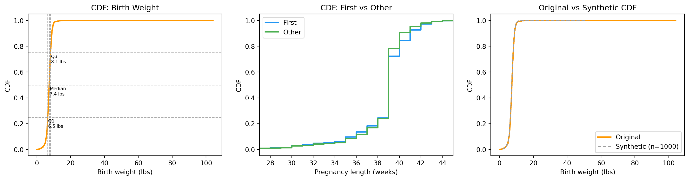
fig, axes = plt.subplots(1, 3, figsize=(15, 4))

# 1. CDF with quartile annotations
ax = axes[0]
ax.plot(wgt_cdf_all.xs, wgt_cdf_all.ps, color="#FF9800", linewidth=2)
for p, label in [(0.25, "Q1"), (0.5, "Median"), (0.75, "Q3")]:
    x = wgt_cdf_all.value(p)
    ax.axvline(x, color=COLORS["neutral"], linestyle="--", linewidth=1)
    ax.axhline(p, color=COLORS["neutral"], linestyle="--", linewidth=1)
    ax.annotate(f"{label}\n{x:.1f} lbs", xy=(x, p),
                xytext=(x + 0.3, p - 0.08), fontsize=7)
ax.set_xlabel("Birth weight (lbs)")
ax.set_ylabel("CDF")
ax.set_title("CDF: Birth Weight")

# 2. Group comparison
ax = axes[1]
ax.plot(prg_cdf_first.xs, prg_cdf_first.ps,
        color=COLORS["first"], linewidth=2, label="First")
ax.plot(prg_cdf_other.xs, prg_cdf_other.ps,
        color=COLORS["other"], linewidth=2, label="Other")
ax.set_xlabel("Pregnancy length (weeks)")
ax.set_ylabel("CDF")
ax.set_title("CDF: First vs Other")
ax.legend()
ax.set_xlim(27, 45)

# 3. Synthetic vs original
ax = axes[2]
ax.plot(wgt_cdf_all.xs, wgt_cdf_all.ps,
        color="#FF9800", linewidth=2, label="Original")
ax.plot(synthetic_cdf.xs, synthetic_cdf.ps,
        color=COLORS["neutral"], linewidth=1.5, linestyle="--",
        label="Synthetic (n=1000)")
ax.set_xlabel("Birth weight (lbs)")
ax.set_ylabel("CDF")
ax.set_title("Original vs Synthetic CDF")
ax.legend()

plt.tight_layout()
plt.show()

Birth weight CDF with quartiles, pregnancy-length CDFs by group, and synthetic data from the empirical CDF.

---

18.9 Exercises

1. Build a CDF for birth weight. What is the median? What is the IQR?
2. Plot CDFs for first vs other babies. What do you notice?
3. Write percentile_rank(cdf, value) returning the percentile of a given value.
4. Write percentile(cdf, p) returning the value at a given percentile.
5. Use the inverse CDF to generate 500 synthetic birth weights. Plot them vs the original CDF.

---

18.10 Glossary

CDF — F(x) = P(X \leq x); fraction of data at or below x.

percentile — value below which a given percentage of observations fall.

median — 50th percentile; robust to outliers.

quartile — 25th, 50th, or 75th percentile.

IQR — Q3 − Q1; spread of the middle 50% of the data.

inverse CDF — given p, returns x such that F(x) = p.

robust statistic — not strongly affected by outliers.