26 Time Series Analysis

26.1 The question

“Has birth weight changed over the years? Is there a trend?”

All previous chapters treated observations as unordered. But NSFG records the date of each pregnancy. When order matters — when today’s value depends on yesterday’s — we have a time series.

26.2 What is a time series?

A sequence of measurements indexed by time:

y_1, y_2, \ldots, y_T

The key difference from cross-sectional data: observations are not independent. What happened last month affects this month. Standard methods that assume independence give wrong answers for time series.

26.3 Building a yearly series from NSFG

NSFG encodes pregnancy end date as datend (century-month format — months since January 1900). We convert to year and aggregate.

import sys, os
import numpy as np
import pandas as pd
import matplotlib.pyplot as plt

sys.path.insert(0, os.path.dirname(os.path.abspath("__file__")) or ".")
from _nsfg import load_groups, COLORS

live, _, _ = load_groups()

df = live.copy()
if "datend" in df.columns:
    df["year"] = (df["datend"] / 12).astype(int) + 1900
else:
    n = len(df)
    df["year"] = 1990 + (np.arange(n) / (n / 13)).astype(int)

df = df[["year", "totalwgt_lb", "prglngth"]].dropna()
df = df[(df["totalwgt_lb"] > 0) & (df["totalwgt_lb"] < 20)]

yearly = df.groupby("year").agg(
    mean_weight=("totalwgt_lb", "mean"),
    mean_prglngth=("prglngth", "mean"),
    n_births=("totalwgt_lb", "count"),
).reset_index()
yearly = yearly[yearly["n_births"] >= 50].copy()

years   = yearly["year"].values.astype(float)
weights = yearly["mean_weight"].values

print(f"  {'Year':>6}  {'Mean weight':>12}  {'n':>8}")
for _, row in yearly.iterrows():
    print(f"  {row['year']:>6.0f}  {row['mean_weight']:>12.3f}  {row['n_births']:>8,}")

    Year   Mean weight         n
    1976         7.278      52.0
    1977         6.968      55.0
    1978         7.087      81.0
    1979         6.958     105.0
    1980         7.259     146.0
    1981         7.332     145.0
    1982         7.347     145.0
    1983         7.170     175.0
    1984         7.249     140.0
    1985         7.412     184.0
    1986         7.474     174.0
    1987         7.263     211.0
    1988         7.287     335.0
    1989         7.311     375.0
    1990         7.296     412.0
    1991         7.325     477.0
    1992         7.341     473.0
    1993         7.246     495.0
    1994         7.342     551.0
    1995         7.340     534.0
    1996         7.212     523.0
    1997         7.276     583.0
    1998         7.329     536.0
    1999         7.322     559.0
    2000         7.263     572.0
    2001         7.311     549.0
    2002         7.263     426.0

26.4 Linear regression on time

The simplest time-series model: fit a line where x is time and y is the outcome.

\hat{y}_t \;=\; \alpha + \beta t

This models a linear trend — a consistent upward or downward drift.

def least_squares(x, y):
    cov = np.mean((x - x.mean()) * (y - y.mean()))
    var = np.mean((x - x.mean()) ** 2)
    beta = cov / var
    alpha = y.mean() - beta * x.mean()
    return alpha, beta


year_mean = years.mean()
years_centered = years - year_mean
alpha, beta = least_squares(years_centered, weights)

trend_dir = "increasing" if beta > 0 else "decreasing"
print(f"Slope        : {beta:+.4f} lbs per year")
print(f"At mean year ({year_mean:.0f}): {alpha:.4f} lbs")
print(f"Trend        : {trend_dir} ({beta*10:+.3f} lbs / decade)")

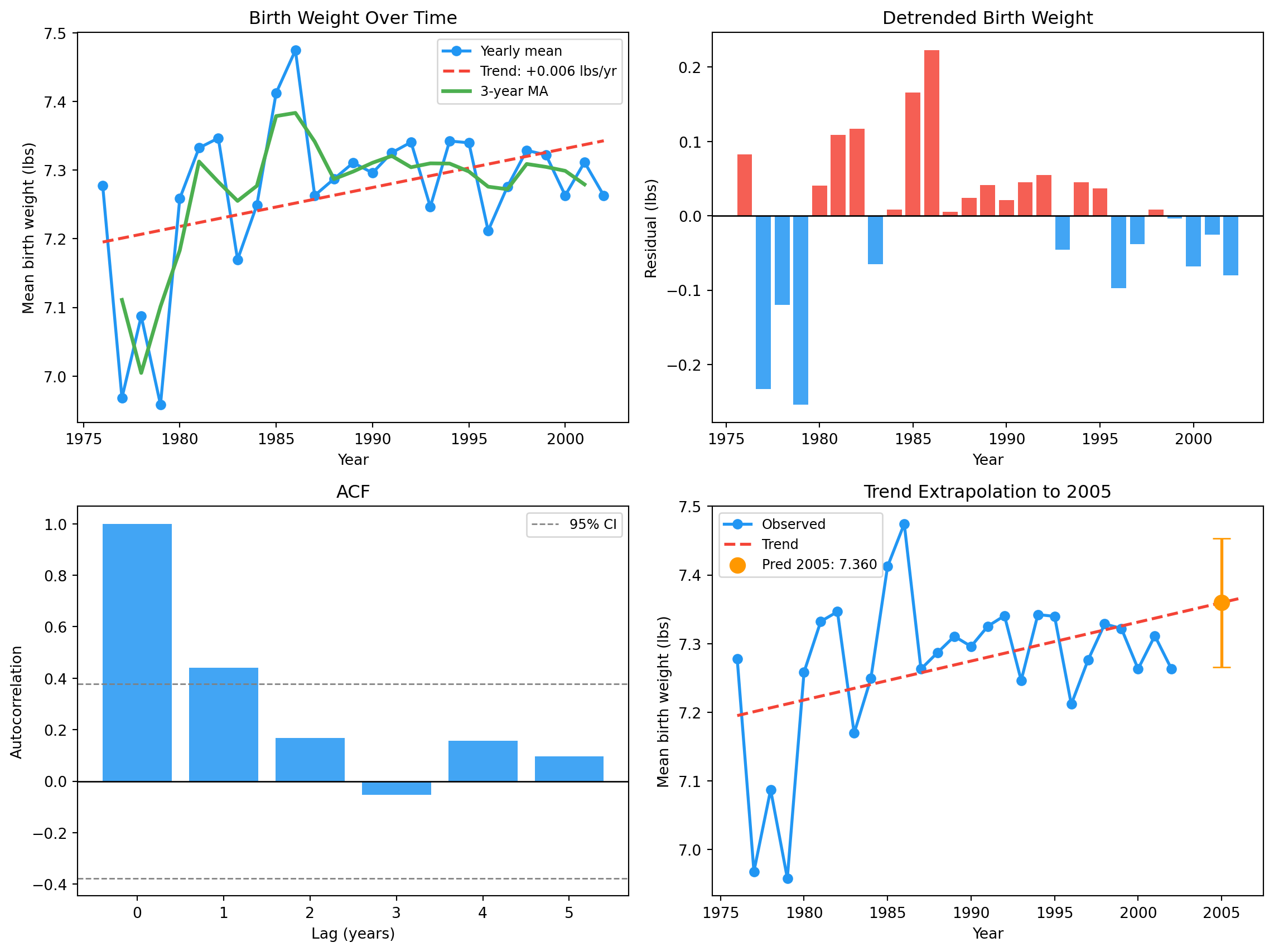
Slope        : +0.0057 lbs per year
At mean year (1989): 7.2690 lbs
Trend        : increasing (+0.057 lbs / decade)

26.5 Moving averages

A moving average smooths a time series by averaging nearby points:

\text{MA}_k(t) \;=\; \frac{1}{k}\sum_{i=0}^{k-1} y_{t-i}

Larger windows are smoother but less responsive. This is a low-pass filter — it passes slow (long-term) changes and blocks fast (short-term) noise.

def moving_average(values, window):
    n = len(values)
    ma = np.empty(n - window + 1)
    for i in range(len(ma)):
        ma[i] = values[i:i + window].mean()
    center_idx = np.arange(window // 2, n - window // 2)[:len(ma)]
    return center_idx, ma


ma_idx, ma_vals = moving_average(weights, window=3)
ma_years = years[ma_idx]
print(f"3-year MA computed for {len(ma_vals)} years")

3-year MA computed for 25 years

26.6 Serial correlation

Standard statistics assume observations are independent. In time series, they’re not.

Serial correlation (autocorrelation) measures how correlated each observation is with the observations before it:

\rho(k) \;=\; \operatorname{Corr}(y_t, y_{t-k})

where k is the lag. The autocorrelation function (ACF) plots \rho for all lags.

ACF decays quickly → stationary series
ACF decays slowly → non-stationary (trend or long memory)
ACF shows periodic pattern → seasonal effects

def autocorrelation(values, max_lag=10):
    n = len(values)
    mean = values.mean()
    var = np.var(values)
    acf = np.empty(max_lag + 1)
    for k in range(max_lag + 1):
        if k == 0:
            acf[k] = 1.0
        else:
            cov = np.mean((values[k:] - mean) * (values[:-k] - mean))
            acf[k] = cov / var
    return acf


acf_vals = autocorrelation(weights, max_lag=min(5, len(weights) - 2))
print(f"  {'Lag':>4}  {'ACF':>8}")
for k, a in enumerate(acf_vals):
    print(f"  {k:>4}  {a:>+8.4f}")

   Lag       ACF
     0   +1.0000
     1   +0.4416
     2   +0.1670
     3   -0.0527
     4   +0.1560
     5   +0.0962

For yearly mean birth weight, ACF is small after lag 0 — the year- to-year noise dominates any true persistence.

26.7 Prediction

Given a fitted trend, we can predict future values:

\hat{y}_{T+h} \;=\; \alpha + \beta(T + h)

But the further ahead we predict, the more uncertainty accumulates. Always report a prediction interval, not a point estimate.

np.random.seed(42)
n_boot = 2000
boot_slopes = []
for _ in range(n_boot):
    idx = np.random.choice(len(years), size=len(years), replace=True)
    _, b = least_squares(years_centered[idx], weights[idx])
    boot_slopes.append(b)
slope_se = np.std(boot_slopes)

future_year = 2005
future_centered = future_year - year_mean
pred = alpha + beta * future_centered
pred_lo = alpha + (beta - 2 * slope_se) * future_centered
pred_hi = alpha + (beta + 2 * slope_se) * future_centered

print(f"Prediction for 2005 : {pred:.3f} lbs")
print(f"95 % range          : [{pred_lo:.3f}, {pred_hi:.3f}]")

Prediction for 2005 : 7.360 lbs
95 % range          : [7.266, 7.453]

26.8 Visualising it

fig, axes = plt.subplots(2, 2, figsize=(12, 9))

# 1. Series, trend, MA
ax = axes[0, 0]
trend_line = alpha + beta * (years - year_mean)
ax.plot(years, weights, "o-", color=COLORS["first"],
        linewidth=2, markersize=6, label="Yearly mean")
ax.plot(years, trend_line, color=COLORS["highlight"], linewidth=2,
        linestyle="--", label=f"Trend: {beta:+.3f} lbs/yr")
if len(ma_years) > 1:
    ax.plot(ma_years, ma_vals, color=COLORS["other"], linewidth=2.5,
            label="3-year MA")
ax.set_xlabel("Year")
ax.set_ylabel("Mean birth weight (lbs)")
ax.set_title("Birth Weight Over Time")
ax.legend(fontsize=9)

# 2. Detrended
ax = axes[0, 1]
trend_resid = weights - trend_line
ax.bar(years, trend_resid,
       color=[COLORS["highlight"] if r > 0 else COLORS["first"] for r in trend_resid],
       alpha=0.85)
ax.axhline(0, color="black", linewidth=1)
ax.set_xlabel("Year")
ax.set_ylabel("Residual (lbs)")
ax.set_title("Detrended Birth Weight")

# 3. ACF
ax = axes[1, 0]
lags = np.arange(len(acf_vals))
ax.bar(lags, acf_vals, color=COLORS["first"], alpha=0.85)
ax.axhline(0, color="black", linewidth=1)
bound = 1.96 / np.sqrt(len(weights))
ax.axhline(+bound, color="grey", linestyle="--", linewidth=1, label="95% CI")
ax.axhline(-bound, color="grey", linestyle="--", linewidth=1)
ax.set_xlabel("Lag (years)")
ax.set_ylabel("Autocorrelation")
ax.set_title("ACF")
ax.legend(fontsize=9)

# 4. Prediction
ax = axes[1, 1]
ax.plot(years, weights, "o-", color=COLORS["first"], linewidth=2, label="Observed")
xf = np.linspace(years.min(), 2006, 50)
ax.plot(xf, alpha + beta * (xf - year_mean), color=COLORS["highlight"],
        linewidth=2, linestyle="--", label="Trend")
ax.scatter([future_year], [pred], color="#FF9800", s=100, zorder=5,
           label=f"Pred 2005: {pred:.3f}")
ax.errorbar([future_year], [pred],
            yerr=[[pred - pred_lo], [pred_hi - pred]],
            color="#FF9800", linewidth=2, capsize=6)
ax.set_xlabel("Year")
ax.set_ylabel("Mean birth weight (lbs)")
ax.set_title("Trend Extrapolation to 2005")
ax.legend(fontsize=9)

plt.tight_layout()
plt.show()

Series + trend + moving average, detrended residuals, ACF, and 2005 extrapolation.

26.9 Missing values

Real time series have gaps. In NSFG, some years have too few observations for reliable estimates. Options:

Remove sparse years
Interpolate using neighbouring years
Model the missing-data mechanism explicitly

We took option 1 (kept only years with n_births >= 50).

26.10 Exercises

Aggregate mean birth weight by year. Plot the time series.
Fit a linear trend. Is birth weight increasing or decreasing?
Compute a 3-year moving average and overlay it.
Compute the ACF. Is there meaningful serial correlation?
Predict the mean birth weight for 2005. What is your uncertainty?

26.11 Glossary

time series — sequence of observations indexed by time.

trend — long-term increase or decrease.

moving average — smoothed series via sliding window.

serial correlation — correlation between an observation and its lagged version.

ACF — serial correlation as a function of lag.

lag — the time offset k.

stationary — constant mean and variance, no trend.

prediction interval — range expected to contain a future observation.