4 Conditional Probability

4.1 Why Conditional Probability?

A rapid test for a disease is described as 95% accurate. You take the test. It comes back positive. How worried should you be?

Most people say: 95% chance I have it. The correct answer — which we will derive — might be closer to 9%. The difference is dramatic, and it comes entirely from ignoring one piece of information: how common is the disease in the first place?

This is the central insight of conditional probability. Probabilities are not static — they must be revised when new information arrives. The three tools that make this precise are:

The Multiplication Rule — probability of a sequence of events
The Total Probability Theorem — breaking a complex event into simpler scenarios
Bayes’ Rule — working backwards from observed evidence to hidden causes

These three tools, combined, are the foundation of inference — the entire field of reasoning from data to conclusions.

4.2 1. Revised Beliefs

4.2.1 The Intuition

Imagine a town registry of 1000 residents. You pick one at random.

Before any information: P(\text{person is under 18}) \approx 0.25.
New information: the person is married.
After the information: P(\text{person is under 18} \mid \text{married}) is now much smaller — perhaps 0.01.

The new information did not change the world. It changed what we know about it, which forces a revision of our probability. Conditional probability is the formal machinery for this revision.

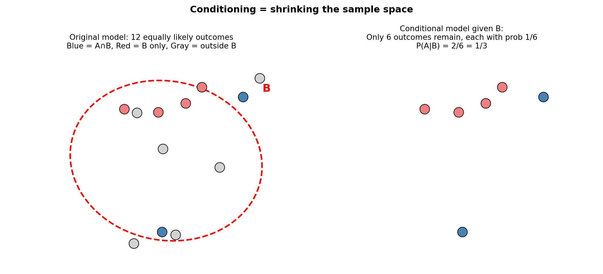
4.2.2 Shrinking the Sample Space

When we learn that event B has occurred, two things happen:

Elimination: every outcome not in B becomes impossible.
Re-normalisation: the remaining outcomes in B must now sum to probability 1, so their relative weights are preserved but scaled up.

import matplotlib.pyplot as plt
import matplotlib.patches as mpatches
import numpy as np

fig, axes = plt.subplots(1, 2, figsize=(11, 5))

# Left: original sample space with 12 equally likely outcomes
ax = axes[0]
np.random.seed(0)
xs = np.random.uniform(0.1, 0.9, 12)
ys = np.random.uniform(0.1, 0.9, 12)

# Mark 6 as "in B" and 2 of those as "in A ∩ B"
in_B = [False]*12
in_AB = [False]*12
for i in [1, 3, 5, 7, 9, 11]:
    in_B[i] = True
for i in [3, 7]:
    in_AB[i] = True

for i, (x, y) in enumerate(zip(xs, ys)):
    color = 'steelblue' if in_AB[i] else ('lightcoral' if in_B[i] else 'lightgray')
    ax.scatter(x, y, c=color, s=160, zorder=3, edgecolors='black', linewidths=0.8)

ellipse_B = mpatches.Ellipse((0.55, 0.5), 0.65, 0.75, angle=15,
                               fill=False, edgecolor='red', linewidth=2, linestyle='--')
ax.add_patch(ellipse_B)
ax.text(0.88, 0.82, 'B', fontsize=14, color='red', fontweight='bold')
ax.set_xlim(0, 1); ax.set_ylim(0, 1)
ax.set_title('Original model: 12 equally likely outcomes\nBlue = A∩B, Red = B only, Gray = outside B',
             fontsize=10)
ax.axis('off')

# Right: conditional model — only B remains
ax2 = axes[1]
xs_B = [xs[i] for i in range(12) if in_B[i]]
ys_B = [ys[i] for i in range(12) if in_B[i]]
in_AB_B = [in_AB[i] for i in range(12) if in_B[i]]

for x, y, ab in zip(xs_B, ys_B, in_AB_B):
    color = 'steelblue' if ab else 'lightcoral'
    ax2.scatter(x, y, c=color, s=160, zorder=3, edgecolors='black', linewidths=0.8)

ax2.set_xlim(0, 1); ax2.set_ylim(0, 1)
ax2.set_title('Conditional model given B:\nOnly 6 outcomes remain, each with prob 1/6\nP(A|B) = 2/6 = 1/3',
              fontsize=10)
ax2.axis('off')

plt.suptitle('Conditioning = shrinking the sample space', fontsize=12, fontweight='bold')
plt.tight_layout()
plt.show()

4.3 2. The Definition

Conditional Probability

The conditional probability of event A given that event B has occurred is:

P(A \mid B) = \frac{P(A \cap B)}{P(B)}

Requirements: P(B) > 0. (We cannot condition on something that cannot happen.)

This is a definition, not a theorem. We choose this formula because it captures the intuition of restricting attention to the outcomes inside B and rescaling.

Sanity checks:

P(B \mid B) = \frac{P(B \cap B)}{P(B)} = 1 — if we know B occurred, it is certain. ✓
P(\emptyset \mid B) = \frac{P(\emptyset)}{P(B)} = 0 — the impossible event stays impossible. ✓
P(\Omega \mid B) = \frac{P(B)}{P(B)} = 1 — something must happen. ✓

The conditional probability law P(\cdot \mid B) is itself a valid probability law — it satisfies all three Kolmogorov axioms. This means every theorem we proved from the axioms (complement rule, inclusion-exclusion, union bound, etc.) holds for conditional probabilities too.

4.4 3. A Worked Example: The 4-Sided Die

Roll a 4-sided die twice. Sample space: 16 equally likely outcomes.

Event B: the minimum of the two rolls is exactly 2. B = \{(2,2),(2,3),(2,4),(3,2),(4,2)\}, \quad P(B) = \frac{5}{16}

omega = {(i, j) for i in range(1, 5) for j in range(1, 5)}
n = len(omega)

B = {(i, j) for i, j in omega if min(i, j) == 2}
print(f"B = {sorted(B)}")
print(f"P(B) = {len(B)}/{n} = {len(B)/n:.4f}")

B = [(2, 2), (2, 3), (2, 4), (3, 2), (4, 2)]
P(B) = 5/16 = 0.3125

Question A: P(\max = 1 \mid \min = 2)

If the minimum is 2, the maximum cannot be 1 — they would both have to be 1, but then the minimum would be 1, not 2.

P(M=1 \mid Z=2) = \frac{P(\{M=1\} \cap B)}{P(B)} = \frac{0}{5/16} = 0

Question B: P(\max = 3 \mid \min = 2)

# Method 1: formal formula
A = {(i, j) for i, j in omega if max(i, j) == 3}
A_and_B = A & B
print(f"A ∩ B (max=3 AND min=2) = {sorted(A_and_B)}")
print(f"P(A ∩ B) = {len(A_and_B)}/{n}")
print(f"P(max=3 | min=2) = {len(A_and_B)/n:.4f} / {len(B)/n:.4f} = {len(A_and_B)/len(B):.4f}")

# Method 2: directly count within B
outcomes_in_B_with_max3 = [(i,j) for i,j in B if max(i,j) == 3]
print(f"\nMethod 2 (count within B): {outcomes_in_B_with_max3}")
print(f"P(max=3 | min=2) = {len(outcomes_in_B_with_max3)}/{len(B)} = {len(outcomes_in_B_with_max3)/len(B):.4f}")

A ∩ B (max=3 AND min=2) = [(2, 3), (3, 2)]
P(A ∩ B) = 2/16
P(max=3 | min=2) = 0.1250 / 0.3125 = 0.4000

Method 2 (count within B): [(2, 3), (3, 2)]
P(max=3 | min=2) = 2/5 = 0.4000

Both methods give \frac{2}{5}. Method 2 makes the intuition concrete: once we know B occurred, we live in a new universe of 5 outcomes, and 2 of them have maximum = 3.

4.5 4. The Multiplication Rule

Rearranging the definition of conditional probability gives:

P(A \cap B) = P(B) \cdot P(A \mid B) = P(A) \cdot P(B \mid A)

This is the Multiplication Rule for two events. It extends to any number of events:

General Multiplication Rule

P(A_1 \cap A_2 \cap \cdots \cap A_n) = P(A_1) \cdot P(A_2 \mid A_1) \cdot P(A_3 \mid A_1 \cap A_2) \cdots P(A_n \mid A_1 \cap \cdots \cap A_{n-1})

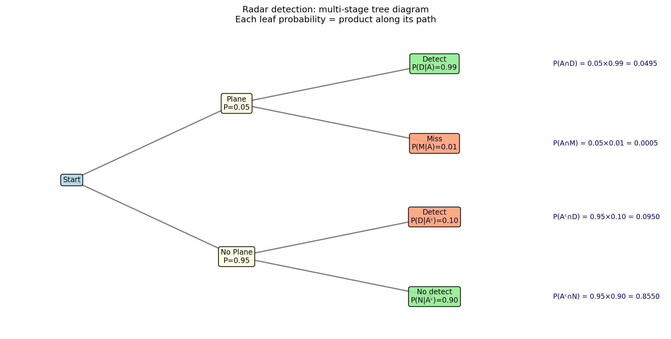
Tree diagram interpretation: each factor is the probability of one branch, given all previous branches were taken. To get the probability of a leaf (a complete outcome), multiply along the path.

4.5.1 Example: Drawing Cards Without Replacement

A standard deck has 52 cards. Draw 3 cards without replacement. What is the probability all three are aces?

Let A_i = “the i-th card is an ace.”

P(A_1 \cap A_2 \cap A_3) = P(A_1) \cdot P(A_2 \mid A_1) \cdot P(A_3 \mid A_1 \cap A_2) = \frac{4}{52} \cdot \frac{3}{51} \cdot \frac{2}{50} = \frac{24}{132600} \approx 0.000181

import numpy as np

# Analytical
p_analytical = (4/52) * (3/51) * (2/50)
print(f"Analytical: {p_analytical:.6f}")

# Simulation
np.random.seed(42)
n_trials = 500_000
deck = np.array([1]*4 + [0]*48)  # 1 = ace, 0 = non-ace
count = 0
for _ in range(n_trials):
    draw = np.random.choice(deck, size=3, replace=False)
    if draw.sum() == 3:
        count += 1

print(f"Simulation:  {count / n_trials:.6f}")

Analytical: 0.000181
Simulation:  0.000166

4.6 5. Multi-Stage Models: Radar Detection

Conditional probabilities are the natural building blocks of multi-stage experiments. Consider a radar system:

Stage 1 (reality): Is a plane present?
- P(\text{plane}) = 0.05, P(\text{no plane}) = 0.95
Stage 2 (radar response): Does the radar detect something?
- P(\text{detect} \mid \text{plane}) = 0.99 — hits
- P(\text{detect} \mid \text{no plane}) = 0.10 — false alarms

import matplotlib.pyplot as plt
import matplotlib.patches as mpatches

fig, ax = plt.subplots(figsize=(12, 6))
ax.axis('off')

# Node positions
nodes = {
    'root': (0.1, 0.5),
    'plane': (0.35, 0.75),
    'no_plane': (0.35, 0.25),
    'detect_p': (0.65, 0.88),
    'miss_p': (0.65, 0.62),
    'detect_np': (0.65, 0.38),
    'miss_np': (0.65, 0.12),
}

labels = {
    'root': 'Start',
    'plane': 'Plane\nP=0.05',
    'no_plane': 'No Plane\nP=0.95',
    'detect_p': 'Detect\nP(D|A)=0.99',
    'miss_p': 'Miss\nP(M|A)=0.01',
    'detect_np': 'Detect\nP(D|Aᶜ)=0.10',
    'miss_np': 'No detect\nP(N|Aᶜ)=0.90',
}

leaf_probs = {
    'detect_p': f'P(A∩D) = 0.05×0.99 = {0.05*0.99:.4f}',
    'miss_p':   f'P(A∩M) = 0.05×0.01 = {0.05*0.01:.4f}',
    'detect_np':f'P(Aᶜ∩D) = 0.95×0.10 = {0.95*0.10:.4f}',
    'miss_np':  f'P(Aᶜ∩N) = 0.95×0.90 = {0.95*0.90:.4f}',
}

colors = {
    'root': 'lightblue', 'plane': 'lightyellow', 'no_plane': 'lightyellow',
    'detect_p': 'lightgreen', 'miss_p': 'lightsalmon',
    'detect_np': 'lightsalmon', 'miss_np': 'lightgreen',
}

edges = [
    ('root', 'plane'), ('root', 'no_plane'),
    ('plane', 'detect_p'), ('plane', 'miss_p'),
    ('no_plane', 'detect_np'), ('no_plane', 'miss_np'),
]

for a, b in edges:
    ax.annotate('', xy=nodes[b], xytext=nodes[a],
                arrowprops=dict(arrowstyle='->', color='gray', lw=1.5))

for k, (x, y) in nodes.items():
    ax.text(x, y, labels[k], ha='center', va='center', fontsize=9,
            bbox=dict(boxstyle='round', facecolor=colors[k], alpha=0.9))

for k, prob_text in leaf_probs.items():
    x, y = nodes[k]
    ax.text(x + 0.18, y, prob_text, ha='left', va='center',
            fontsize=8.5, color='darkblue')

ax.set_title('Radar detection: multi-stage tree diagram\n'
             'Each leaf probability = product along its path', fontsize=11)
plt.tight_layout()
plt.show()

The key numbers from this model:

# Stage probabilities
P_A  = 0.05   # plane present
P_Ac = 0.95   # no plane

P_D_given_A  = 0.99  # detect | plane
P_D_given_Ac = 0.10  # detect | no plane (false alarm)

# Multiplication rule: leaf probabilities
P_A_and_D  = P_A  * P_D_given_A
P_Ac_and_D = P_Ac * P_D_given_Ac

print(f"P(plane AND detect)    = {P_A_and_D:.4f}")
print(f"P(no plane AND detect) = {P_Ac_and_D:.4f}")

P(plane AND detect)    = 0.0495
P(no plane AND detect) = 0.0950

4.7 6. Total Probability Theorem

The radar example shows a general pattern. If A_1, A_2, \ldots, A_n partition \Omega (disjoint, exhaustive, each with P(A_i) > 0), then any event B can be broken into pieces:

B = (B \cap A_1) \cup (B \cap A_2) \cup \cdots \cup (B \cap A_n)

Since the pieces are disjoint, additivity gives:

Total Probability Theorem

P(B) = \sum_{i=1}^n P(A_i) \cdot P(B \mid A_i)

Interpretation: P(B) is a weighted average of the conditional probabilities P(B \mid A_i), weighted by how likely each scenario A_i is.

# Total probability of radar detection
P_D = P_A_and_D + P_Ac_and_D
print(f"P(detect) = P(A)·P(D|A) + P(Aᶜ)·P(D|Aᶜ)")
print(f"         = {P_A}×{P_D_given_A} + {P_Ac}×{P_D_given_Ac}")
print(f"         = {P_A_and_D:.4f} + {P_Ac_and_D:.4f}")
print(f"         = {P_D:.4f}")

P(detect) = P(A)·P(D|A) + P(Aᶜ)·P(D|Aᶜ)
         = 0.05×0.99 + 0.95×0.1
         = 0.0495 + 0.0950
         = 0.1445

14.45% of the time the radar goes off — mostly due to false alarms, because planes are rare.

4.8 7. Bayes’ Rule

We now have all the pieces. Given that the radar detected something, what is the probability a plane is actually there?

This is inference: observing an effect (radar signal) and reasoning about its cause (plane or not).

Bayes’ Rule

Given a partition A_1, \ldots, A_n of \Omega and an observed event B:

P(A_i \mid B) = \frac{P(A_i) \cdot P(B \mid A_i)}{\displaystyle\sum_{j=1}^n P(A_j) \cdot P(B \mid A_j)}

P(A_i) — prior: belief about scenario A_i before observing B
P(B \mid A_i) — likelihood: how probable is B under scenario A_i
P(A_i \mid B) — posterior: revised belief after observing B

Bayes’ Rule is not a new theorem — it is just the definition of conditional probability, with the numerator expanded by the Multiplication Rule and the denominator by the Total Probability Theorem.

# Bayes' Rule: P(plane | detection)
P_A_given_D = P_A_and_D / P_D
print(f"P(plane | detect) = P(A∩D) / P(D)")
print(f"                  = {P_A_and_D:.4f} / {P_D:.4f}")
print(f"                  = {P_A_given_D:.4f}  ({P_A_given_D*100:.1f}%)")

P(plane | detect) = P(A∩D) / P(D)
                  = 0.0495 / 0.1445
                  = 0.3426  (34.3%)

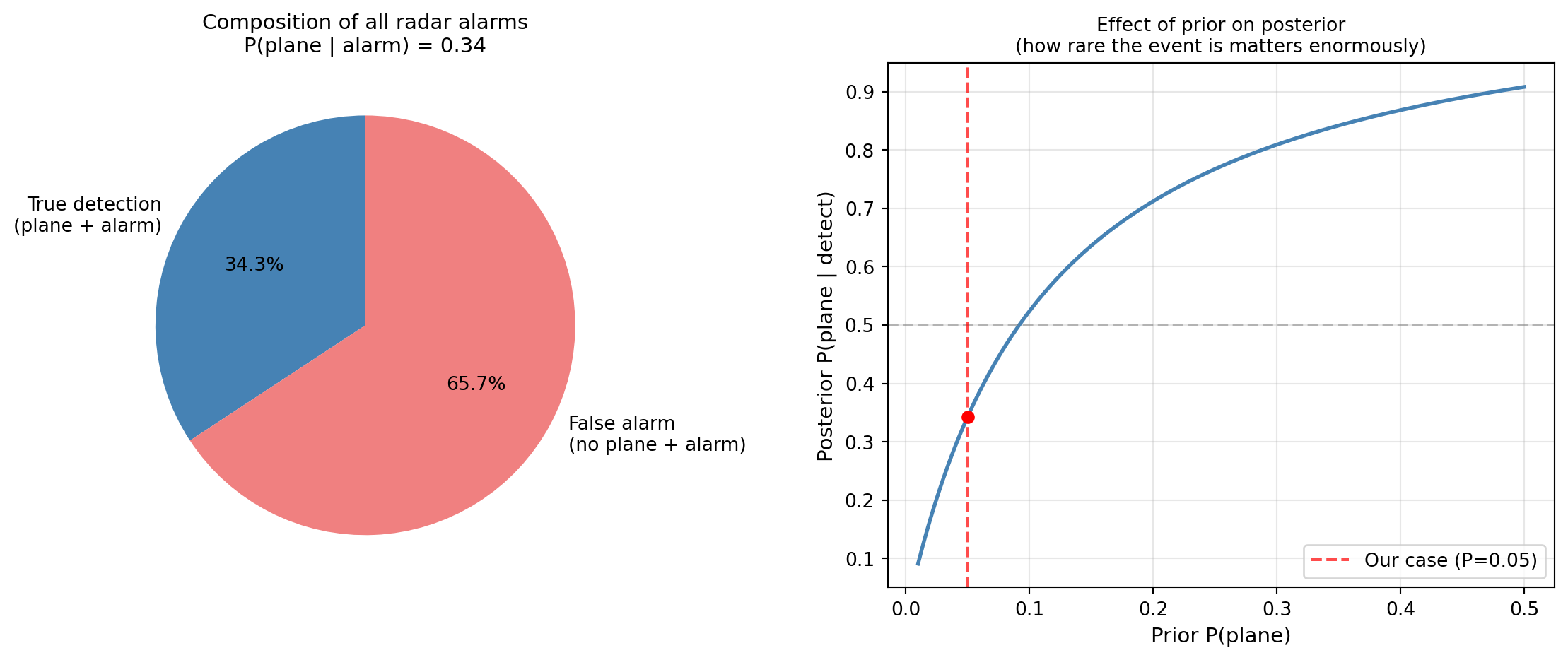
The paradox of low priors: even though the radar is 99% accurate at detecting real planes and has only a 10% false alarm rate, when it goes off there is only a 34% chance a plane is actually there.

Why? Because planes are rare (P = 5\%). The large pool of “no plane” situations generates many false alarms even at 10% — far outnumbering the true detections.

import matplotlib.pyplot as plt

fig, axes = plt.subplots(1, 2, figsize=(12, 5))

# Left: visualise the populations
labels_pie = ['True detection\n(plane + alarm)', 'False alarm\n(no plane + alarm)']
sizes = [P_A_and_D, P_Ac_and_D]
colors = ['steelblue', 'lightcoral']
axes[0].pie(sizes, labels=labels_pie, colors=colors, autopct='%1.1f%%',
            startangle=90, textprops={'fontsize': 10})
axes[0].set_title(f'Composition of all radar alarms\n'
                  f'P(plane | alarm) = {P_A_given_D:.2f}', fontsize=11)

# Right: posterior vs prior for different prior values
priors = np.linspace(0.01, 0.5, 200)
posteriors = (priors * P_D_given_A) / (priors * P_D_given_A + (1 - priors) * P_D_given_Ac)
axes[1].plot(priors, posteriors, color='steelblue', lw=2)
axes[1].axhline(0.5, color='gray', linestyle='--', alpha=0.5)
axes[1].axvline(0.05, color='red', linestyle='--', alpha=0.7, label='Our case (P=0.05)')
axes[1].scatter([0.05], [P_A_given_D], color='red', zorder=5)
axes[1].set_xlabel('Prior P(plane)', fontsize=11)
axes[1].set_ylabel('Posterior P(plane | detect)', fontsize=11)
axes[1].set_title('Effect of prior on posterior\n(how rare the event is matters enormously)',
                  fontsize=10)
axes[1].legend()
axes[1].grid(True, alpha=0.3)

plt.tight_layout()
plt.show()

4.9 8. Back to the Medical Test

Now we can answer the opening question properly.

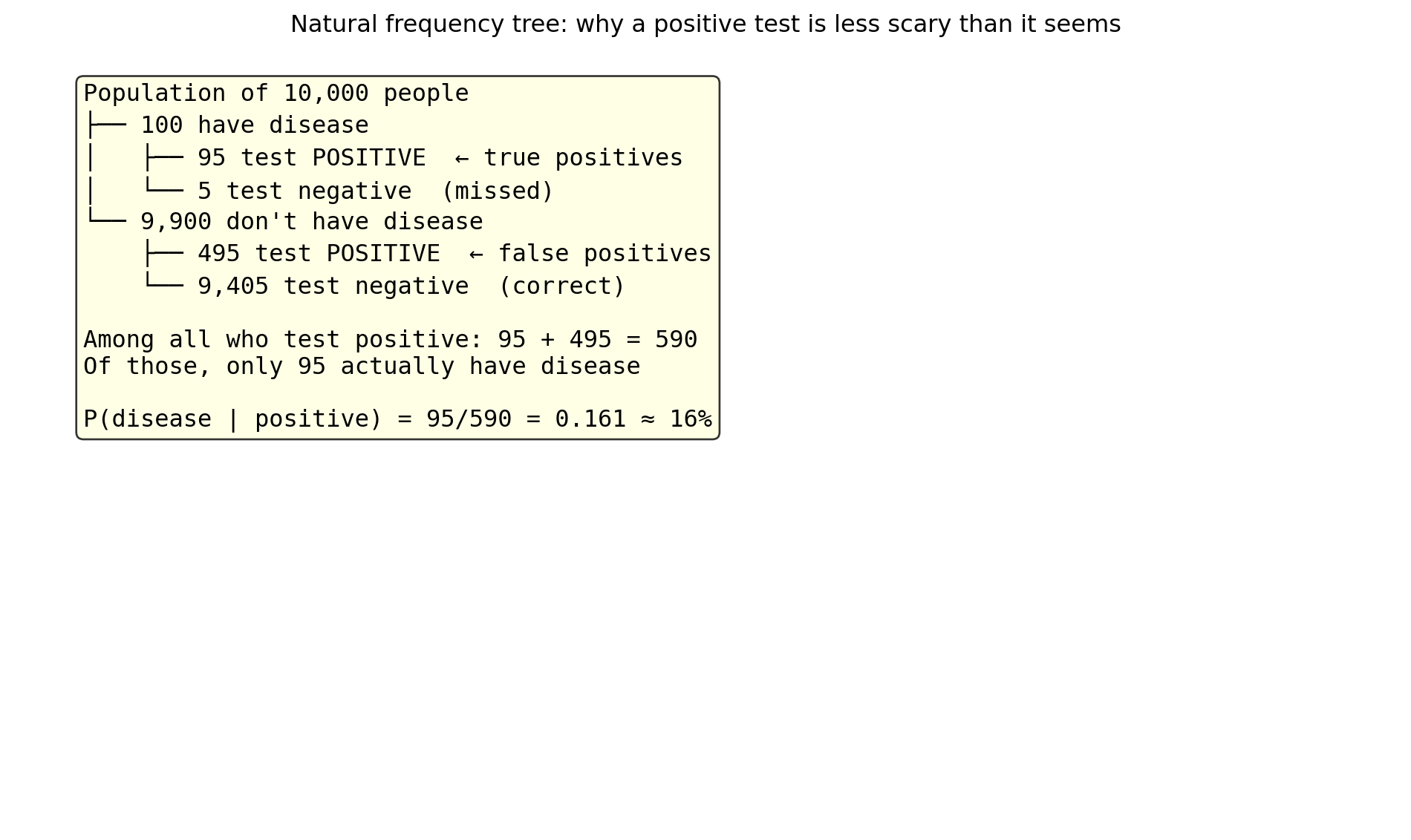
A disease affects 1% of the population. A test is 95% accurate:

P(\text{positive} \mid \text{disease}) = 0.95 — sensitivity
P(\text{positive} \mid \text{no disease}) = 0.05 — false positive rate

You test positive. What is P(\text{disease} \mid \text{positive})?

P_disease     = 0.01   # prior: 1% of population has it
P_pos_given_D = 0.95   # sensitivity
P_pos_given_H = 0.05   # false positive rate (H = healthy)

# Total probability of testing positive
P_pos = P_disease * P_pos_given_D + (1 - P_disease) * P_pos_given_H
print(f"P(positive) = {P_disease}×{P_pos_given_D} + {1-P_disease}×{P_pos_given_H} = {P_pos:.4f}")

# Bayes: posterior
P_D_given_pos = (P_disease * P_pos_given_D) / P_pos
print(f"\nP(disease | positive) = {P_D_given_pos:.4f}  ({P_D_given_pos*100:.1f}%)")

P(positive) = 0.01×0.95 + 0.99×0.05 = 0.0590

P(disease | positive) = 0.1610  (16.1%)

import matplotlib.pyplot as plt

# Visualise with a frequency tree (natural frequencies approach)
fig, ax = plt.subplots(figsize=(10, 6))
ax.axis('off')

population = 10000
has_disease = int(population * P_disease)       # 100
no_disease  = population - has_disease          # 9900

true_pos  = int(has_disease * P_pos_given_D)    # 95
false_neg = has_disease - true_pos              # 5
false_pos = int(no_disease * P_pos_given_H)     # 495
true_neg  = no_disease - false_pos              # 9405

text = (
    f"Population of {population:,} people\n"
    f"├── {has_disease} have disease\n"
    f"│   ├── {true_pos} test POSITIVE  ← true positives\n"
    f"│   └── {false_neg} test negative  (missed)\n"
    f"└── {no_disease:,} don't have disease\n"
    f"    ├── {false_pos} test POSITIVE  ← false positives\n"
    f"    └── {true_neg:,} test negative  (correct)\n\n"
    f"Among all who test positive: {true_pos} + {false_pos} = {true_pos + false_pos}\n"
    f"Of those, only {true_pos} actually have disease\n\n"
    f"P(disease | positive) = {true_pos}/{true_pos + false_pos} = {true_pos/(true_pos+false_pos):.3f} ≈ {P_D_given_pos*100:.0f}%"
)

ax.text(0.05, 0.95, text, transform=ax.transAxes, fontsize=12,
        verticalalignment='top', fontfamily='monospace',
        bbox=dict(boxstyle='round', facecolor='lightyellow', alpha=0.8))
ax.set_title('Natural frequency tree: why a positive test is less scary than it seems',
             fontsize=12)
plt.tight_layout()
plt.show()

Out of 10,000 people who take the test, 590 test positive — but only 95 of them actually have the disease. That is 16%, not 95%.

The result is so counterintuitive because the false positives (495) swamp the true positives (95). The disease is rare, so the large healthy population produces many false alarms even at a 5% false positive rate.

4.10 9. Conditional Probability Satisfies the Axioms

A key fact: for any fixed event B with P(B) > 0, the function Q(A) = P(A \mid B) is itself a valid probability law. It satisfies:

Non-negativity: P(A \mid B) = \frac{P(A \cap B)}{P(B)} \ge 0 since both numerator and denominator are non-negative. ✓
Normalization: P(\Omega \mid B) = \frac{P(\Omega \cap B)}{P(B)} = \frac{P(B)}{P(B)} = 1. ✓
Additivity: if A_1 \cap A_2 = \emptyset, then (A_1 \cap B) \cap (A_2 \cap B) = \emptyset, so P(A_1 \cup A_2 \mid B) = P(A_1 \mid B) + P(A_2 \mid B). ✓

This means every theorem derived from the axioms — complement rule, monotonicity, inclusion-exclusion, union bound — holds for conditional probabilities too, simply by replacing P(\cdot) with P(\cdot \mid B) everywhere.

4.11 10. Exercises

1. Conditional probability from a table. A company has 200 employees:

	Promoted	Not promoted
Male	40	80
Female	30	50

A randomly chosen employee is selected.

What is P(\text{promoted})?
What is P(\text{promoted} \mid \text{female})?
What is P(\text{female} \mid \text{promoted})?
Is promotion independent of gender? (Hint: check whether P(\text{promoted} \mid \text{female}) = P(\text{promoted}).)

2. Multiplication rule. A bag has 5 red balls and 3 blue balls. Draw 3 balls without replacement.

Use the multiplication rule to find P(\text{all three red}).
Use the multiplication rule to find P(\text{first red, second blue, third red}).
Verify (a) by direct counting: how many ways to choose 3 red balls from 5, divided by total ways to choose 3 balls from 8?

3. Total probability theorem. A factory has two machines. Machine A produces 60% of output and has a 3% defect rate. Machine B produces 40% and has a 5% defect rate.

Use the Total Probability Theorem to find P(\text{defective}).
Write a simulation to verify your answer.

4. Bayes’ Rule. Using the factory setup from Exercise 3, a randomly chosen item is found to be defective.

What is P(\text{made by Machine A} \mid \text{defective})?
What is P(\text{made by Machine B} \mid \text{defective})?
Interpret: even though Machine B has a higher defect rate, why might the answer to (a) be large?

5. Medical testing — varying the prior. Using the medical test example (95% sensitivity, 5% false positive rate):

Compute P(\text{disease} \mid \text{positive}) for disease prevalences of 1%, 5%, 10%, and 50%.
Plot the posterior probability as a function of prior prevalence.
At what prevalence does a positive test result in a 50% posterior probability of disease?

6. Sequential Bayes. You take the medical test twice (independently). Both come back positive.

Treat the first test result as establishing a new prior. Apply Bayes’ Rule a second time to find P(\text{disease} \mid \text{two positives}).
Write a simulation to verify.
Compare with the result from a single positive test.