17  Probability Mass Functions

17.1 The problem with histograms

In Chapter 2 we normalised histograms to compare groups of different sizes. But histograms have a hidden problem: the shape changes with bin width.

Try these bin widths for pregnancy length:

• 1 week → clean picture, matches clinical intuition
• 0.5 weeks → noisy, looks random
• 3 weeks → too coarse, merges distinct peaks

There is no objectively correct bin width. This is uncomfortable.

The Probability Mass Function (PMF) solves this for discrete data.

---

17.2 What is a PMF?

A PMF maps each possible value to its probability:

P(X = x) \;=\; \frac{\text{count}(x)}{n}

For pregnancy length (measured in whole weeks), there are about 18 distinct values (27 through 44). The PMF assigns a probability to each one.

No bins. No arbitrary choices. The PMF is the exact empirical distribution.

Key property: probabilities sum to 1.

\sum_x P(X = x) \;=\; 1

---

17.3 Building a PMF from scratch

import sys, os
import numpy as np
import matplotlib.pyplot as plt

sys.path.insert(0, os.path.dirname(os.path.abspath("__file__")) or ".")
from _nsfg import load_groups, COLORS

live, first, other = load_groups()


class Pmf:
    """Probability Mass Function — maps values to probabilities."""

    def __init__(self, values):
        counts: dict = {}
        for v in values:
            if not _is_nan(v):
                counts[v] = counts.get(v, 0) + 1
        total = sum(counts.values())
        self.d: dict = {v: c / total for v, c in counts.items()}

    def prob(self, value, default: float = 0.0) -> float:
        return self.d.get(value, default)

    def values(self):
        return sorted(self.d.keys())

    def probs(self):
        return [self.d[v] for v in self.values()]

    def mean(self) -> float:
        return sum(v * p for v, p in self.d.items())

    def __repr__(self):
        return f"Pmf({len(self.d)} values, mean={self.mean():.3f})"


def _is_nan(v) -> bool:
    try:
        return np.isnan(v)
    except (TypeError, ValueError):
        return False


first_pmf = Pmf(first["prglngth"].dropna().values)
other_pmf = Pmf(other["prglngth"].dropna().values)
print(first_pmf)
print(f"Most probable length (first) : {max(first_pmf.d, key=first_pmf.d.get):.0f} wks")
print(f"Most probable length (other) : {max(other_pmf.d, key=other_pmf.d.get):.0f} wks")

Pmf(31 values, mean=38.601)
Most probable length (first) : 39 wks
Most probable length (other) : 39 wks

That’s it. A PMF is a normalised frequency count.

---

17.4 PMFs reveal what histograms hide

When you plot first vs other babies as PMFs, you see something a histogram smooths over: the distributions have subtly different shapes near 39 weeks.

print(f"  {'Week':>4}   {'First':>7}   {'Other':>7}   {'Diff':>8}")
for week in range(35, 45):
    f = first_pmf.prob(week)
    o = other_pmf.prob(week)
    print(f"  {week:>4}   {f:>7.4f}   {o:>7.4f}   {f-o:>+8.4f}")

  Week     First     Other       Diff
    35    0.0360    0.0321    +0.0039
    36    0.0390    0.0315    +0.0075
    37    0.0471    0.0522    -0.0050
    38    0.0616    0.0707    -0.0091
    39    0.4790    0.5447    -0.0656
    40    0.1215    0.1225    -0.0010
    41    0.0816    0.0479    +0.0336
    42    0.0465    0.0260    +0.0205
    43    0.0197    0.0129    +0.0068
    44    0.0052    0.0049    +0.0004

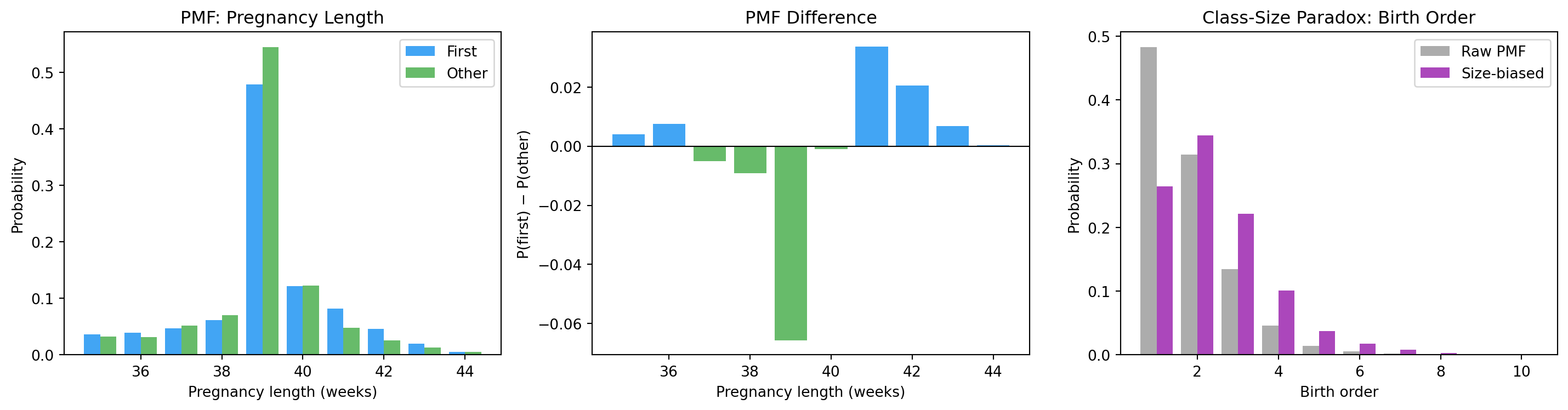
Other babies are slightly more likely to be born at exactly 39 weeks. First babies have a longer right tail. The mean difference is real, but it’s driven by the tail — not a uniform shift of the whole distribution.

---

17.5 Plotting PMFs

Unlike a histogram (bars touching, continuous), a PMF for discrete data is plotted as separated bars or stems — because the gaps between integer values are real: no pregnancy is 38.7 weeks long.

---

17.6 The class size paradox

This is one of the most elegant examples in statistics — a case where the same data gives different answers depending on who you ask.

A college has departments of varying sizes:

Department	Size	# Departments
Small	10	8
Medium	100	2

From the department’s perspective: average class size = (8 × 10 + 2 × 100) / 10 = 28 students.

From the student’s perspective: most students are in large classes; a student picked at random is more likely to be in a 100-person class. average = (80 × 10 + 200 × 100) / 280 ≈ 79 students.

Same college. Same data. Completely different averages. Why?

Because the probability of being in a large class is proportional to the class size itself. The PMF is biased by the very thing we’re measuring.

Formally, if P(X = x) is the unbiased PMF, the size-biased one is:

P(X^* = x) \;=\; \frac{x \cdot P(X = x)}{E[X]}

This is the size-biased distribution, also called the inspection paradox.

# Simulate the college from above
np.random.seed(42)
departments = [10] * 8 + [100] * 2
dept_mean = np.mean(departments)

all_students = []
for size in departments:
    all_students.extend([size] * size)
student_mean = np.mean(all_students)

print(f"Departments view : {dept_mean:.1f} students")
print(f"Students' view   : {student_mean:.1f} students "
      f"({student_mean / dept_mean:.1f}x larger)")

Departments view : 28.0 students
Students' view   : 74.3 students (2.7x larger)

The same paradox applies to NSFG family size: if you ask mothers how many children they have, you oversample mothers with many children (because large families contribute more respondents).

def size_biased(pmf: Pmf) -> Pmf:
    biased = {v: p * v for v, p in pmf.d.items()}
    total = sum(biased.values())
    result = Pmf.__new__(Pmf)
    result.d = {v: c / total for v, c in biased.items()}
    return result


birthord_pmf_raw    = Pmf(live["birthord"].dropna().values)
birthord_pmf_biased = size_biased(birthord_pmf_raw)

print(f"Mean birth order (raw PMF)       : {birthord_pmf_raw.mean():.3f}")
print(f"Mean birth order (size-biased)   : {birthord_pmf_biased.mean():.3f}")
print("A random child 'experiences' a larger family than the average mother reports.")

Mean birth order (raw PMF)       : 1.826
Mean birth order (size-biased)   : 2.418
A random child 'experiences' a larger family than the average mother reports.

---

17.7 Visualising it

fig, axes = plt.subplots(1, 3, figsize=(15, 4))

# 1. PMF comparison
ax = axes[0]
weeks = list(range(35, 45))
first_p = [first_pmf.prob(w) for w in weeks]
other_p = [other_pmf.prob(w) for w in weeks]
x = np.array(weeks)
ax.bar(x - 0.2, first_p, width=0.4, color=COLORS["first"], alpha=0.85, label="First")
ax.bar(x + 0.2, other_p, width=0.4, color=COLORS["other"], alpha=0.85, label="Other")
ax.set_xlabel("Pregnancy length (weeks)")
ax.set_ylabel("Probability")
ax.set_title("PMF: Pregnancy Length")
ax.legend()

# 2. PMF difference
ax = axes[1]
diffs = [first_pmf.prob(w) - other_pmf.prob(w) for w in weeks]
diff_colors = [COLORS["first"] if d > 0 else COLORS["other"] for d in diffs]
ax.bar(weeks, diffs, color=diff_colors, alpha=0.85)
ax.axhline(0, color="black", linewidth=0.8)
ax.set_xlabel("Pregnancy length (weeks)")
ax.set_ylabel("P(first) − P(other)")
ax.set_title("PMF Difference")

# 3. Class-size paradox on NSFG birth order
ax = axes[2]
values = sorted(birthord_pmf_raw.d.keys())
raw    = [birthord_pmf_raw.prob(v)    for v in values]
biased = [birthord_pmf_biased.prob(v) for v in values]
xb = np.array(values)
ax.bar(xb - 0.2, raw,    width=0.4, color=COLORS["neutral"], alpha=0.85, label="Raw PMF")
ax.bar(xb + 0.2, biased, width=0.4, color="#9C27B0",         alpha=0.85, label="Size-biased")
ax.set_xlabel("Birth order")
ax.set_ylabel("Probability")
ax.set_title("Class-Size Paradox: Birth Order")
ax.legend()

plt.tight_layout()
plt.show()

PMFs side-by-side, the first–other difference, and the size-biased birth-order paradox.

---

17.8 Exercises

1. Build a PMF of prglngth for all live births. What is the most common length?
2. Build PMFs for first vs other babies separately. At which week do they differ most?
3. Implement the class size paradox using NSFG family size data.
4. Build a PMF of birth order. What fraction of live births are first babies?
5. What is the mean of the size-biased distribution of birthord? Compare to the raw mean.

---

17.9 Glossary

PMF — maps each value of a discrete variable to its probability.

discrete variable — takes countable values (whole weeks).

size-biased distribution — sampling probability is proportional to value size.

inspection paradox — distribution experienced by a random member differs from the population distribution.

empirical distribution — distribution computed directly from observed data, not a theoretical model.