A different sensor on the motor monitors shock pulses — the high-frequency clicks a damaged ball bearing emits as it rolls past a load zone. On a healthy bearing, these clicks are extremely rare; on a damaged one, they multiply.
You want a maintenance metric: how many shock pulses arrive in a one-hour window?
Try modelling this with the Binomial. You’d need:
n — the number of “trials” per hour. But what is a trial? A nanosecond? A bearing rotation? It depends on how finely you slice time.
p — the probability of a click in one trial. As you slice time finer, n grows and p shrinks.
Yet the expected count per hour — say, \lambda = 3 clicks/hour on a healthy bearing — is a real, measurable physical quantity. It doesn’t depend on how you slice time.
You want a distribution parameterised by \lambda alone, where the trial-counting machinery quietly disappears. That distribution exists, and it’s what the Binomial becomes in exactly this regime.
7.2 Intuition
The Poisson distribution is what the Binomial becomes when:
n \to \infty (the region is sliced into infinitely many trials)
p \to 0 (each trial is vanishingly unlikely)
\lambda = np stays constant (the expected count is fixed by the physics)
The two parameters collapse into one: \lambda, the expected count per region.
7.3 The derivation
Note▶ Show the math — Binomial → Poisson limit
Start from the Binomial PMF and substitute p = \lambda / n:
The magical property: mean equals variance. This single fact is the engine behind every shot-noise calculation in sensors, every queueing model in networks, and every count-based regression in statistics.
7.4 The Poisson has ONE parameter
Distribution
Parameters
Mean
Variance
Mean = Variance?
Binomial(n, p)
n, p
np
np(1-p)
only when p \to 0
Poisson(\lambda)
\lambda
\lambda
\lambda
always
If you measure the mean of a Poisson process, you immediately know its variance.
7.5 Examples across domains
Process
Underlying n
Underlying p
\lambda
Bearing shock pulses
Time slices per hour
P(click in slice)
Clicks per hour
Network packet drops
Packets per minute
P(drop)
Drops per minute
Photon counting
Available photons
P(photon hits photosite)
Expected electrons per exposure
Defects on a surface
Surface micro-cells
P(defect per cell)
Defects per m²
Earthquakes in a region
“Trial” stress events
P(release per event)
Events per year
Huge n, tiny p, moderate \lambda — the Poisson regime.
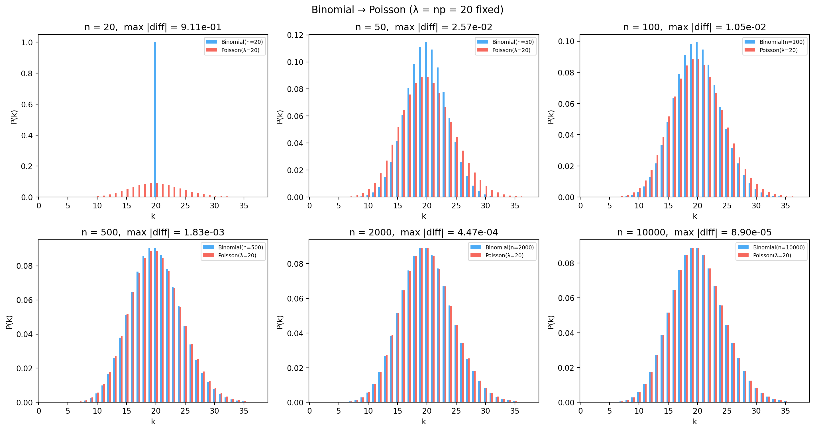
7.6 Watching Binomial → Poisson
import numpy as npimport matplotlib.pyplot as pltfrom scipy.stats import binom, poissonnp.random.seed(42)lambda_fixed =20fig, axes = plt.subplots(2, 3, figsize=(15, 8))n_values = [20, 50, 100, 500, 2000, 10000]for ax, n inzip(axes.flat, n_values): p = lambda_fixed / n # p shrinks as n grows; np = λ stays constant k = np.arange(max(0, int(lambda_fixed -4* np.sqrt(lambda_fixed))),int(lambda_fixed +4* np.sqrt(lambda_fixed)) +1) binom_pmf = binom.pmf(k, n, p) pois_pmf = poisson.pmf(k, lambda_fixed) ax.bar(k -0.15, binom_pmf, width=0.3, color="#2196F3", alpha=0.8, label=f"Binomial(n={n})") ax.bar(k +0.15, pois_pmf, width=0.3, color="#F44336", alpha=0.8, label=f"Poisson(λ={lambda_fixed})") max_diff = np.max(np.abs(binom_pmf - pois_pmf)) ax.set_title(f"n = {n}, max |diff| = {max_diff:.2e}") ax.set_xlabel("k") ax.set_ylabel("P(k)") ax.legend(fontsize=7)plt.suptitle(f"Binomial → Poisson (λ = np = {lambda_fixed} fixed)", fontsize=13)plt.tight_layout()plt.show()
By n \approx 100, the difference is already negligible. By n =
10\,000, the two distributions are indistinguishable.
7.7 Back to the bearing
For the healthy bearing with \lambda = 3 clicks/hour:
So observing 0 clicks in an hour is uncommon (5 % of healthy hours) but not alarming. Observing 10 clicks in an hour is roughly a 1-in-1000 event under the healthy model — strong evidence the bearing state has changed.
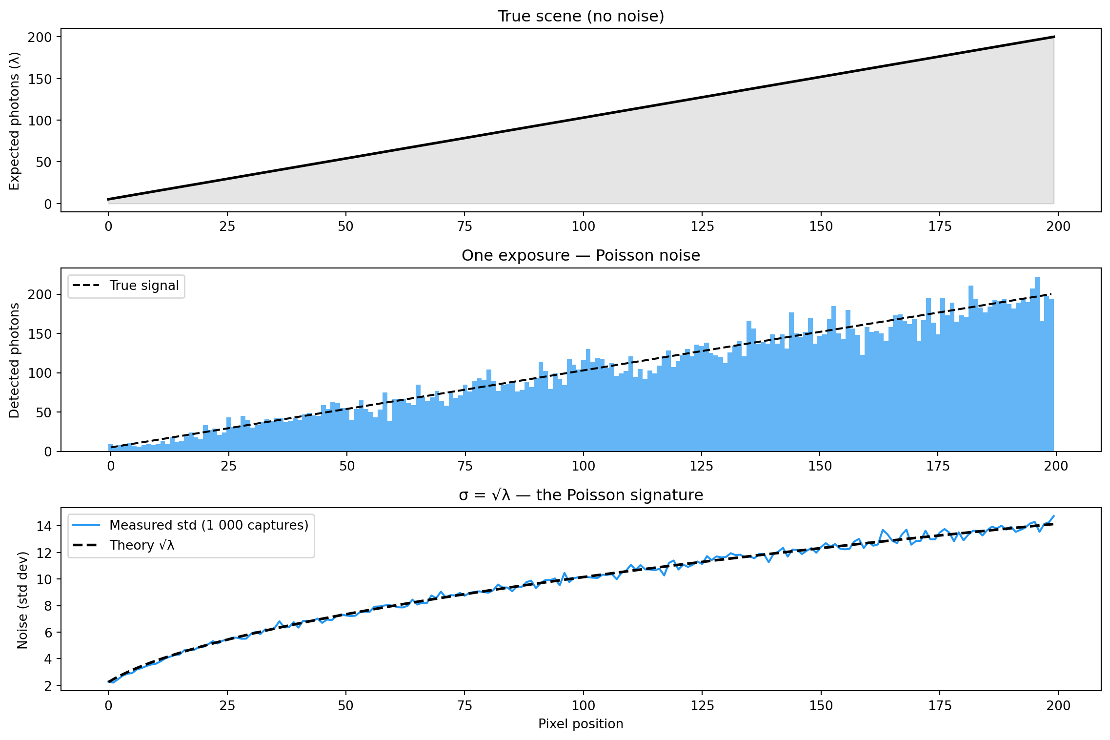
7.8 Poisson noise along a gradient
The variance-equals-mean property has a direct consequence for sensors: in a brightness gradient, dark pixels are relatively noisier than bright pixels.
Top: noiseless ground truth. Middle: one Poisson capture (more visible noise on the dark left). Bottom: measured std exactly tracks σ = √λ.
Dark pixels (left, \lambda \approx 5) have noise \sigma \approx
\sqrt 5 \approx 2.2 — relative noise \approx 45 \%. Bright pixels (right, \lambda \approx 200) have \sigma \approx 14.1 — relative noise \approx 7 \%. Noise grows in absolute terms but shrinks relative to signal: SNR = \sqrt{\lambda}.
7.9 Why Poisson is the right model for photon counting
A typical LED emits ~10^{18} photons per second. The probability that any specific photon reaches a 6 µm × 6 µm photosite is vanishingly small. But the product \lambda = np — determined by illumination, reflectance, exposure time, and sensor area — sits in the range of tens to thousands.
This is exactly the Poisson regime: enormous n, tiny p, moderate \lambda. The Poisson model is not an approximation here — it is the physically correct distribution for photon counting.
7.10 Exercises
For \lambda = 20, plot Binomial(n, \lambda/n) vs Poisson PMFs at n = 50, 100, 1000. Plot max |\Delta| vs n on a log-log scale.
For \lambda \in \{1, 5, 10, 50, 200\} verify by simulation that \sigma \approx \sqrt{\lambda}.
The Anscombe transform f(x) = 2\sqrt{x + 3/8} stabilises Poisson variance. Simulate Poisson data at \lambda \in \{5, 50,
500\}, apply the transform, and confirm the post-transform std is approximately 1 across all three.
7.11 Glossary
Poisson distribution — count of rare independent events; P(k) = \lambda^k e^{-\lambda}/k!.
\lambda — expected count per region.
shot noise — the Poisson noise in photon-counting (or any similar) processes.